1. Introduction

Data association stands as a pivotal technology in radar data processing, enabling the accurate identification of true plots and tracks by establishing connections between radar measurements at different time instances. Conventional methods focus on predicting track values, applying specific criteria to filter relevant plots, and utilizing these plots for further filtering [1, 2, 3, 4, 5]. Nonetheless, these algorithms are highly sensitive to sensor inaccuracies, environmental clutter, and target motion dynamics. To address these challenges, numerous advanced algorithms have been developed [6, 7, 8, 9]. For instance, the Truncated Joint Probability Data Association Filter (JPDAF) introduced in [3] effectively filters clutter by leveraging target motion characteristics. Fan et al. [4] tackles association issues in environments with uncertain measurement errors and motion models by integrating fuzzy recursive least squares filtering with JPDAF, ensuring robust tracking. Qin et al. [7] employs the DBSCAN algorithm and Sequential Random Sample Consensus (RANSAC) to preprocess measurement data, significantly reducing computational demands. With the advent of artificial intelligence, researchers have incorporated AI techniques into data association, yielding promising results [10, 11, 12]. While these methods show efficacy in specific scenarios, they remain rooted in traditional frameworks, necessitating the use of filters for data processing. This approach assumes a known system model, a condition often unattainable in real-world environments.

Reinforcement Learning (RL) [20, 21, 22], a groundbreaking AI technique, has evolved over decades, producing notable methodologies such as Q-learning [13, 14, 15], dynamic programming [16, 17, 18], Policy Gradients [19], and Deep Q-Networks (DQN) [23, 24]. At its core, RL involves a machine learning autonomously in an unfamiliar environment under predefined rules, with actions aligned to the real world and feedback provided through rewards or penalties, culminating at a designated endpoint. In essence, the target data association process seeks to identify true plots generated by the target track, organizing them chronologically to form a complete track. This process parallels the quest for an optimal path and can be likened to a game of Snake, where the machine adapts to the target environment governed by motion-based rules. Thus, theoretically, RL is well-suited to address target data association challenges.

In real-world scenarios, where the target system model is unknown and association results are influenced by environmental clutter, sensor errors, and target maneuvers, this paper introduces a novel data association network architecture based on RL. First, a policy network is designed to predict the association probabilities between measurements and their potential source targets, utilizing RL's dynamic exploration capabilities and the long-term memory of LSTM networks [25]. Next, the Bayesian network analyzes the order of multi-order least squares curve fitting for the current track, predicting the next plot position using least squares curve fitting. The input Bayesian recursive function then calculates the reward value for each plot. Finally, tailored mechanisms are proposed, such as the dynamic ring gate screening mechanism for partial clutter suppression, trajectory consistency-based error correction module.

The paper is structured as follows: Section 2 designs the policy network architecture of the algorithm and explains the definition methods for the state space and action space; Section 3 defines and analyzes the reward function; Section 4 introduces the design concepts of the dynamic ring gate screening mechanism and the error correction module; Section 5 trains the network using extensive simulation data, tests its performance, and provides analysis; Section 6 summarizes the algorithm's strengths and weaknesses and explores future research directions.

Figure 1 Policy network.

2. Policy Network Design and Modeling

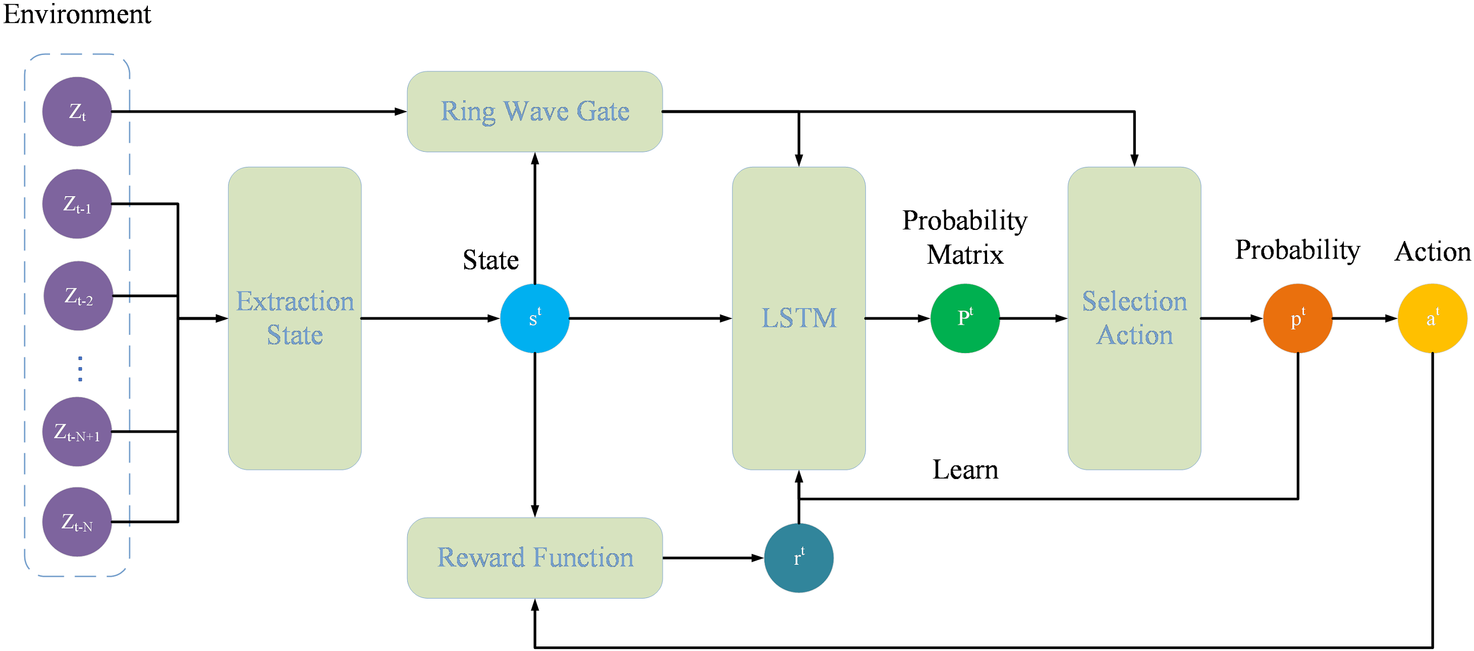
During the correlation of data, sensors capture measurement information in a predefined temporal order. This information includes both authentic target markers and extraneous noise caused by sensor disruptions, environmental conditions, and similar factors. Occasionally, the positions of certain noise elements and genuine target markers in the measurement data may closely align at a specific time, complicating the accurate identification of target-originated markers. Consequently, this paper proposes a policy network capable of dynamically predicting the association probability of points, as illustrated in Figure 1. In scenarios devoid of prior knowledge, the architecture initially employs a strategic network to determine the likelihood of association between the target and measurements, proceeding to link the marker with the greatest probability.

When objects move, they exhibit inertia. This inherent property ensures that the movement patterns of a target remain consistent over short periods. Leveraging this consistency, it's feasible to pinpoint the points that originate from a target by analyzing its movement trajectory, thereby facilitating the precise alignment of measurements with the target. The trajectory of a target is not depicted by isolated points at individual moments but is rather approximated by a series of points over successive intervals. This paper therefore designs a "sliding-window" state, that is, the state of the points associated with the previous $N$ moments. $N$ is the "window" and the size of $N$ is given by the sampling interval of sensor and clutter density. Usually, the larger the sampling interval is, the smaller $N$ is, and vice versa. And the stronger the clutter density, the greater the amount of data to be processed, and the higher the computational load on the hardware, resulting in a smaller $N$, and vice versa.

As shown in Figure 1, $Z_{t-N}$ is the set of measurements when $t-N$, and $s^t$ is the state consisting of points in $\{Z_{t-1},Z_{t-2},\dots ,Z_{t-N}\}$ originating from the target when $t$. Suppose $z_i^{t-N}=\left[\begin{array}{c}{x}_i^{t-N}\\ y_i^{t-N}\end{array}\right]$ is the point in $Z_{t-N}$. $x_i^{t-N}$ and $y_i^{t-N}$ are the positions of $x$ and $y$ axes in the Cartesian coordinate, respectively. If $s^t$ consists of $\{z_i^{t-1},z_i^{t-2},\dots ,z_i^{t-N}\}$, the expression of $s^t$ is as follows:

The construction of states dictates that every state comprises points linked to the preceding $N$ intervals. However, at the initiation of the association process, the agent's initial state must be drawn from the measurement data of the prior $N$ intervals. Consequently, this study introduces an Initial State Extraction mechanism tailored for the agent. Given the random dispersion of clutter, assembling clutter across $N$ successive intervals into a unified track poses a significant challenge. Thus, the mechanism stipulates that a fundamental requirement for identifying an agent is the presence of target-derived points across $N$ consecutive intervals. The operational sequence of this mechanism is illustrated as follows:

As previously mentioned, the action space is composed of the points associated with the agent. The designed learning framework in this study is segmented into a training phase and a testing phase. Throughout the training phase, the agent endeavors to discover the most effective strategy that closely aligns with the target's movement patterns through iterative experimentation. This phase incorporates a Selection Action module known as Random Choice, where the agent picks a random probability value from $P^t$ for a point to facilitate training. During the testing phase, the agent utilizes the insights gained to link points accurately. This phase features a Selection Action module referred to as Argmax Choice, where the agent identifies and selects the point from $P^t$ with the greatest probability value for the purpose of association.

3. Reward Function Definition

This paper introduces a novel reward function designed to evaluate the efficacy of actions chosen in a given state by calculating their true merit. The essence of this function lies in its ability to determine the reward of an action by integrating the anticipated position of the target, as forecasted by the least squares method, into a Bayesian recursive framework at the present moment. The order of the least squares method, crucial for the accuracy of this prediction, is dynamically ascertained by the insights provided by a Bayesian network.

The target's trajectory is characterized by a spectrum of motion patterns, including but not limited to Constant Velocity (CV), Coordinate Turn (CT), and Constant Acceleration (CA). In the tapestry of real-world scenarios, a target's journey may weave through various motion models, rendering the use of a static least squares order inadequate for capturing the nuanced dynamics of its path. To address this, a "sliding window" approach is employed, which, anchored in the current state, forecasts the optimal least squares order capable of modeling the target's motion over a span of $N$ moments. Drawing inspiration from the Bayesian network model outlined in reference [26], an $M$-category Bayesian network is architected, where $M$ symbolizes the stratification of least squares orders into distinct classes. A modest $M$ may fail to encapsulate the full gamut of potential motion trajectories, whereas an excessive $M$ could erode the model's resilience, leading to significant discrepancies in the fitted results. The network ingests the current state as its input and yields the probabilities for each order class as its output, with the least squares order being the one crowned with the highest probability.

Leveraging the predicted order $g$, the least squares method [27] fits the state data to forecast the target's position. The fitted state ${\tilde{s}}^t$ and predicted position ${\tilde{z}}^t$ are defined as: ${\tilde{s}}^t=\left[\begin{array}{c}{\tilde{X}}^t\\ {\tilde{Y}}^t\end{array}\right]$, ${\tilde{z}}^t=\left[\begin{array}{c}{\tilde{x}}^t\\ {\tilde{y}}^t\end{array}\right]$, where the components are calculated through:

The coefficient matrices $W_x$ and $W_y$ are derived from the least squares solution:

where $M_t$ is the design matrix constructed from time terms up to order $g$:

Finally, the reward function $r^t$ is defined via the Bayesian recursive framework [7]:

where $z_i^t$ is the point $i$ selected from the measurement data $Z^t$ when $t$. $K_t\left(Z^t\right)$ is the clutter intensity when $t$, namely $K_t\left(Z^t\right)=\frac{{\text{num}}_{z^t}}{TS}$. In the measurement data $Z^t$, the number of points is ${\text{num}}_{z^t}$. The area of sensor detection region is $TS$. $R$ is the covariance matrix of measurement, which is also the detection error of the sensor.

4. Special Mechanism

4.1 Dynamic Ring Gate Screening Mechanism

The points originating from the target are inherently produced by it and must adhere to its motion dynamics. By leveraging the target's maximum speed $v\_max$ and minimum speed $v\_min$, the annular region of possible points can be delineated, enabling the identification of all potential traces generated by the target. However, these points are subject to the sensor's detection inaccuracy ${\sigma }_v$. Consequently, the speed must dynamically adjust in response to variations in detection error, ensuring alignment with the evolving uncertainty introduced by the sensor's limitations.

$$v\_max=v\_max+\frac{{\sigma }_v^2}{T\_sample}$$

$$v\_min=v\_min-\frac{{\sigma }_v^2}{T\_sample}$$

Figure 2 Dynamic ring gate screening.

Depicted in Figure 2, a target is traversing the monitored zone, with the sensor capturing nine distinct traces at this instance. Upon examining the ring-shaped gating boundary in the illustration, it is discernible that four of these traces are probable candidates for having been generated by the target, namely $z_1,z_2,z_3$ and $z_4$.

Based on the basic information of the target and the sensor, the Ring Wave Gate Screening mechanism eliminates some of the clutter from the measurement data, which not only increases the possibility of selecting the points originating from the target, but also saves the computational resources of policy network.

Utilizing essential details about the target and the sensor, the dynamic ring gate screening mechanism filters out extraneous noise from the measurement dataset. This process not only boosts the probability of detecting traces that stem from the target but also optimizes the computational efficiency of the policy network.

4.2 Error Association Module

In practical settings, targets exhibit a variety of motion patterns, and the network must learn numerous strategies, making comprehensive training unfeasible. When evaluating a new strategy, the unpredictability of the real environment complicates the selection of traces originating from the target. To address this, a module was developed to dynamically refine motion trends during testing, enhancing the limited transferability of RL, as depicted in Figure 3. This module operates by verifying at the test's conclusion; if measurement data persists into the next moment, it signifies an erroneous association, prompting the identification and rectification of the wrongly selected action.

Figure 3 Error correction module.

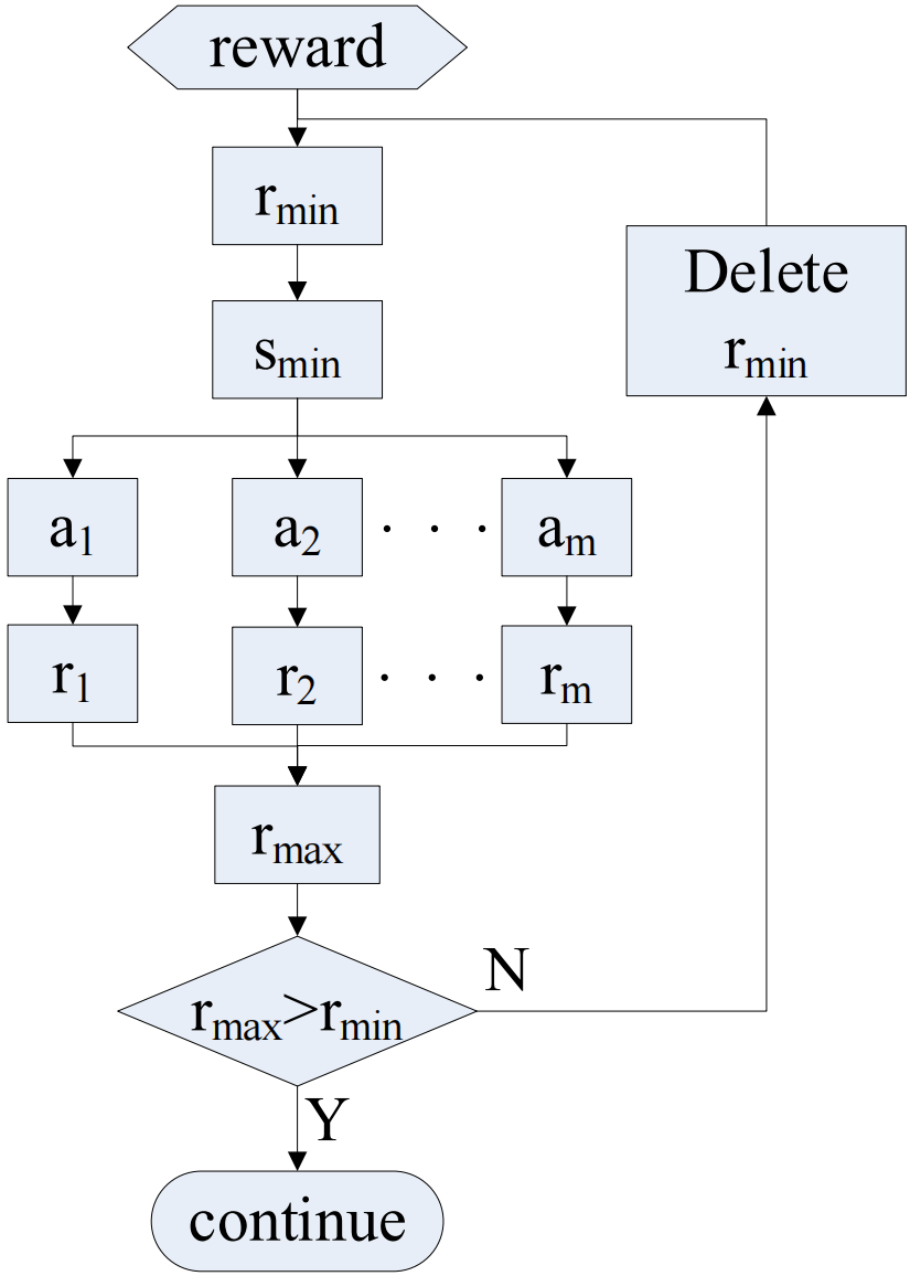
Illustrated in Figure 3, this module unfolds in four distinct stages.

1. Identify the minimum reward value $r\_min$ and its corresponding state $s\_min$ from the set of reward values $reward$.

2. Calculate the reward $r_i$ for each valid action $a_i\left(i=1,2,\dots ,m\right)$ according to equation (13).

3. Judgment: If the maximum reward value $r\_max>r\_min$, select this action to proceed with testing; otherwise, remove $r\_min$ from $reward$ and continue the computation.

4. Examine each reward value within $reward$ in sequence; if no adjustments are necessary, the test concludes.

Throughout the target data association evaluation, this module promptly identifies instances of association errors while bypassing the phase of environmental re-adaptation, thereby boosting the algorithm's applicability and efficiency.

5. Simulation Experiment and Result Analysis

5.2 Result Analysis

The target data association study comprises two distinct phases: the training phase and the evaluation phase. During the training phase, the target's motion duration is 30 seconds. The training dataset is organized into 5 subsets, each corresponding to a specific measurement error ${\sigma }_v=0,10,20,30,40$, with 10,000 data entries per subset. The clutter parameter $\lambda$ is randomly generated within the interval $(0,100)$, and each trajectory's motion model is a random blend of CV, CA, and CT models.

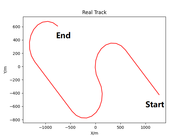
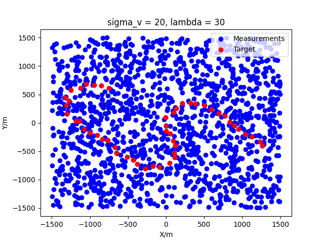
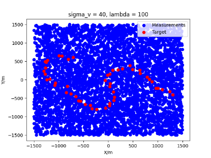
In the evaluation phase, the target's motion spans 50 seconds. The evaluation dataset is segmented into 55 groups based on measurement error ${\sigma }_v=0,10,20,30,40$ and clutter parameter $\lambda =0,10,20,\dots ,90,100$, with each group containing 100 data points, reflecting 100 Monte Carlo simulation trials. The true trajectory is modeled using a combination of CV, CA, CT1, CT2, and CT3 models. Figure 4 depicts the actual trajectory, with the red line indicating the target's true path, "Start" marking the origin, and "End" denoting the destination. Two cases, ${\sigma }_v=20,\lambda =30$ and ${\sigma }_v=40,\lambda =100$, are used as examples to show the distribution of points, as shown in Figure 5.

The state transition matrix and process noise distribution matrix remain consistent for the CV and CA models, namely, $F_{CV},{\Gamma }_{CV},F_{CA},{\Gamma }_{CA}$. For the CT models, $F_{CT}$ and ${\Gamma }_{CT}$ are predominantly stable, with only the parameter $\omega$ in $F_{CT}$ undergoing changes, adhering to a predefined relationship that maps angular rates to distinct maneuver patterns:

Figure 4 Real track.

(a) ${\sigma }_v=20,\lambda =30$

(b) ${\sigma }_v=40,\lambda =100$

Figure 5 Measurement.

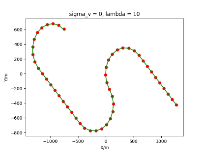
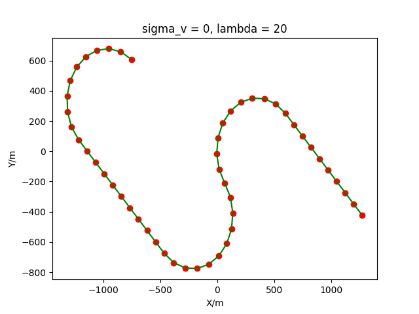
The algorithm is designated as RLDA for short. Through adjustments made in the training phase, the learning rate of the network was set to 0.001, the discount factor to 0.1, and the reward decay to 0.9. Figures 6, 7 and 8 respectively illustrate the association results of the RLDA algorithm under the conditions of ${\sigma }_v=0,20,40$ and $\lambda =0,10,20,\dots ,90,100$. In the RLDA association diagrams, the red markers highlight the true measurements from the target, and the green lines depict the linked trajectories.

Figure 6 Association result of RLDA when ${\sigma }_v$=0.

Figure 7 Association result of RLDA when ${\sigma }_v$=20.

Figure 8 Association result of RLDA when ${\sigma }_v$=40, $\lambda$=100.

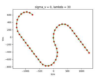
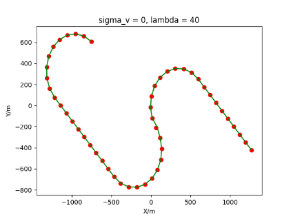
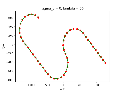
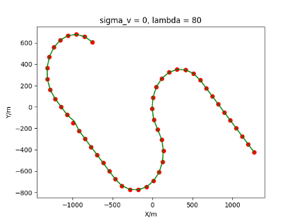
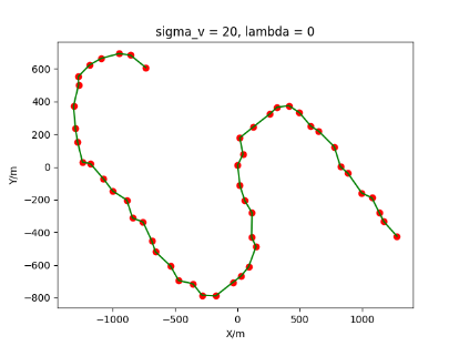
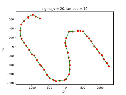
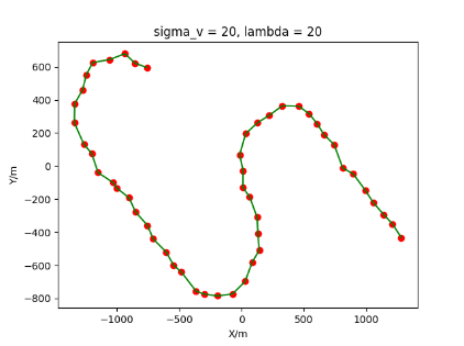
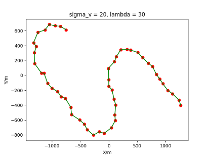
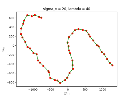
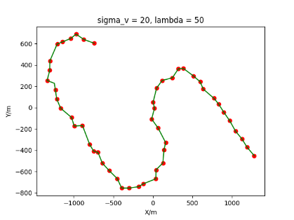
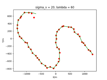
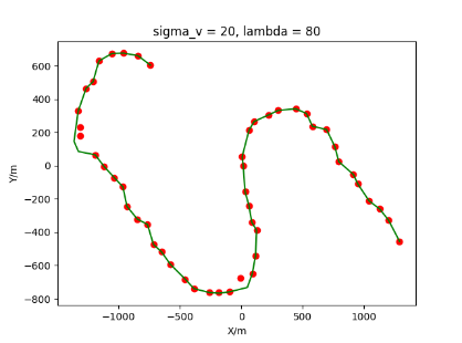
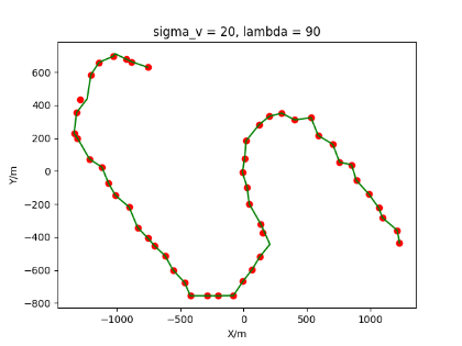
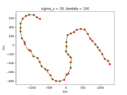
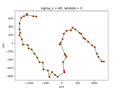
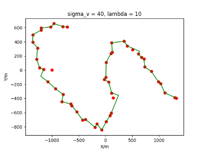
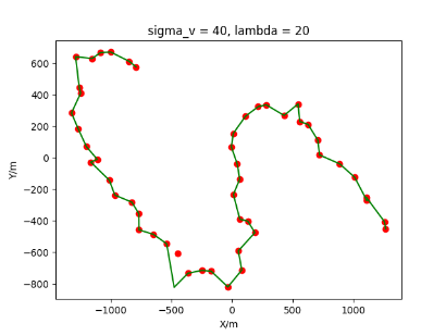
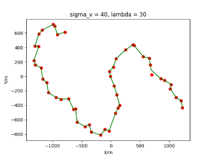
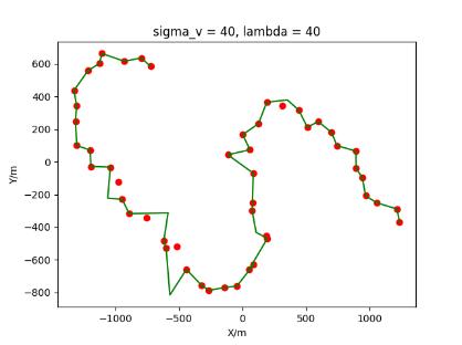
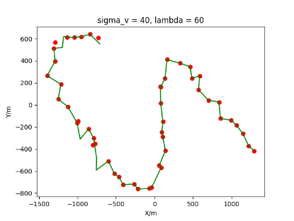
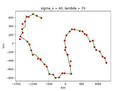
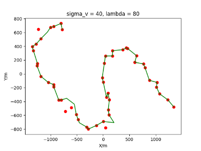
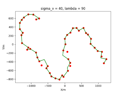
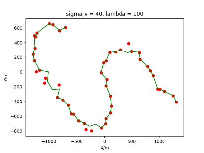
Figures 6, 7 and 8 reveal that as ${\sigma }_v$ and $\lambda$ increase, numerous incorrect associations appear in the results, causing the RLDA algorithm's accuracy to decline. These errors can be grouped into three main types. The first type involves sporadic instances of "mis-selection" during the association process, which do not interfere with subsequent steps. For example, this behavior is observed in the results of ${\sigma }_v=0,\lambda =100$, ${\sigma }_v=20,\lambda =90$, and others. All these figures demonstrate that the agent's future decisions remain unaffected by the mis-selection at the current moment. Moreover, this does not activate the adaptive adjustment mechanism, making it challenging for the agent to detect and rectify the error promptly. However, on a broader scale, this type of error has a negligible impact and does not disrupt the overall association process.

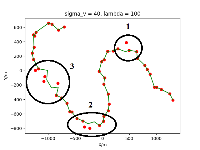
The second type refers to instances where a sequence of incorrect associations arises during a specific phase of the association process. This occurrence is strongly linked to ${\sigma }_v$, especially becoming more frequent during ${\sigma }_v=40$. To explore the underlying causes, the RLDA association results for ${\sigma }_v=40,\lambda =100$ are examined in detail. As illustrated in Figure 9, three segments of erroneous associations are identified, labeled as "1", "2", and "3". Label "1" clearly aligns with the first category, and the associated points better reflect the target's motion trajectory compared to the actual target points, suggesting the agent's decision was more suitable. Labels "2" and "3" both fall into the second category, displaying significant mis-associations due to dense clutter and substantial sensor detection inaccuracies. Since the association process remains continuous and does not activate the adaptive adjustment mechanism, the agent cannot promptly identify and correct these errors. Nonetheless, as depicted in Figure 9, this type of error does not disrupt subsequent associations and has a negligible effect on the overall process.

Figure 9 Association result of RLDA when ${\sigma }_v$=40, $\lambda$=100.

The third type refers to association errors that might emerge as the process nears its conclusion. This behavior is observed in the outcomes of ${\sigma }_v=20,\lambda =60$, ${\sigma }_v=40,\lambda =60$, and similar cases. The cause lies in the target's intense maneuvers, which, under the influence of ${\sigma }_v$

To summarize, as ${\sigma }_v$ and $\lambda$ grow larger, the RLDA algorithm's effectiveness diminishes, and incorrect associations may arise. Nonetheless, the results show that these issues do not compromise the entire process, with only a minor decline in the algorithm's overall performance, while the precision of the association outcomes remains strong. Additionally, this highlights that the RLDA algorithm is capable of effectively handling the association complexities of highly dynamic targets without depending on impractical assumptions, fulfilling the demands of real-world applications.

This research evaluates the RLDA algorithm against the Nearest Neighbor Data Association Filter (NNDAF) [28], the Probability Data Association Filter (PDAF), and the Point-track Association Method with Unknown System Model (USMA) [29]. Given that the simulation involves highly maneuvering targets, the IMM model is incorporated into NNDAF and PDAF, yielding the IMM-NNDAF and IMM-PDAF algorithms, referred to as NNDA and PDA, respectively. To mitigate the inherent limitations of these algorithms, the target's initial position and motion model are predefined. The simulation environment for the USMA algorithm mirrors that of the RLDA algorithm.

At the end of the test, the association accuracy $P$ can be found by comparing the test results with the real points originating from the target, namely $P=\frac{N_{correct}}{N_{all}}$ (The number of real points originating from the target in the association result of agent is $N_{correct}$, and the number of real points originating from the target is $N_{all}$, here $N_{all}=50)$). For each group of data, the average association accuracy $\overline{P}$ can be calculated, namely $\overline{P}=\frac{1}{N_{data}}{\sum }_{i=1}^{N_{data}}{P}_i$ (The number of data in the test set is $N_{data}$, here $N_{data}=100$). The experimental results of test are shown in Tables 1, 2 and 3.

Table 1 Performance comparison of $\overline{P}$ when ${\sigma }_v=0$.

$\overline{P}$		${\sigma }_v=0$
		NNDA	PDA	USMA	RLDA
$\lambda$	0	1	0.731	1	1
	10	0.945	0.684	0.988	1
	20	0.831	0.639	0.960	1
	30	0.650	0.608	0.943	1
	40	0.424	0.555	0.928	0.996
	50	0.213	0.521	0.901	0.992
	60	0.204	0.477	0.887	0.982
	70	0.189	0.449	0.871	0.970
	80	0.114	0.407	0.852	0.964
	90	0.088	0.395	0.828	0.962
	100	0.058	0.358	0.801	0.951

Table 2 Performance comparison of $\overline{P}$ when ${\sigma }_v=20$.

$\overline{P}$		${\sigma }_v=20$
		NNDA	PDA	USMA	RLDA
$\lambda$	0	1	0.5	1	1
	10	0.942	0.490	0.953	1
	20	0.821	0.464	0.932	1
	30	0.552	0.446	0.907	0.996
	40	0.381	0.444	0.871	0.988
	50	0.219	0.413	0.830	0.970
	60	0.198	0.432	0.806	0.962
	70	0.157	0.372	0.771	0.956
	80	0.081	0.401	0.738	0.951
	90	0.054	0.375	0.699	0.938
	100	0.088	0.371	0.665	0.919

Table 3 Performance comparison of $\overline{P}$ when ${\sigma }_v=40$.

$\overline{P}$		${\sigma }_v=40$
		NNDA	PDA	USMA	RLDA
$\lambda$	0	1	0.22	1	1
	10	0.930	0.183	0.891	0.990
	20	0.733	0.207	0.864	0.987
	30	0.440	0.218	0.828	0.969
	40	0.314	0.170	0.790	0.955
	50	0.179	0.194	0.757	0.947
	60	0.158	0.191	0.712	0.935
	70	0.119	0.188	0.676	0.923
	80	0.093	0.167	0.644	0.909
	90	0.056	0.159	0.608	0.897
	100	0.044	0.145	0.537	0.862

The experimental results show that the $\overline{P}$ of RLDA algorithm is inversely proportional to ${\sigma }_v$ and $\lambda$ in terms of the overall trend. However, a closer look at the changes in the data reveals that as ${\sigma }_v$ becomes larger, the effect of $\lambda$ on $\overline{P}$ also becomes larger. When ${\sigma }_v=0,20,40$, $\overline{P}$ decreases by 4.9%, 8.1% and 13.8% during the increase of $\lambda$ from 0 to 100, respectively. Even so, $\overline{P}$ remains above 86%, reflecting the good association performance.

According to the association mechanism of NNDA algorithm, this algorithm is centered on determining the predicted value of track and directly selects the closest point to the center for association. As the results shown in Tables 1, 2 and 3, this algorithm is strongly influenced by clutter. $\overline{P}$ decreases by more than 90% as $\lambda$ increases from 0 to 100. Compared to $\lambda$, this algorithm is minimally affected by ${\sigma }_v$.

As the results shown in Tables 1, 2 and 3, the performance of PDA algorithm gradually decreases as ${\sigma }_v$ and $\lambda$ become larger, and $\overline{P}$ decreases by about 60%.

The USMA algorithm is similar to RLDA algorithm in that both escape the limitations of traditional association algorithms and directly associate the points originating from the target in the real environment. However, the USMA algorithm does not consider the effect of ${\sigma }_v$. As shown in the Tables 1, 2 and 3, when ${\sigma }_v=0,20,40$, $\overline{P}$ decreases by 19.9%, 33.5% and 46.3% during the increase of $\lambda$ from 0 to 100. $\overline{P}$ can only stay above 50% and the association performance of this algorithm is ordinary.

In summary, the RLDA algorithm has the best association performance, followed by the USMA algorithm, and the PDA algorithm and the NNDA algorithm have poor performance. There are too many preconditions to implement the PDA algorithm and NNDA algorithm, but most of these assumptions cannot be predicted in advance (e.g., target motion model, number of targets, etc.). The USMA algorithm is not considered comprehensively enough, and the algorithm performance is unstable when facing the complex real environment.

6. Conclusion

In scenarios where the system model is uncertain, and challenges like intense clutter interference, sensor inaccuracies, and highly maneuvering targets arise, this study introduces a data association algorithm leveraging the LSTM-RL network. This approach moves beyond conventional data association methods by integrating RL technology, creating a unique framework for data association. The architecture combines RL's dynamic exploration capabilities with the long-term memory functions of LSTM networks, enabling it to compute the association probability between the agent and selected measurement points. Target positions are predicted using Bayesian networks and multi-order least squares curve fitting, while reward values are derived from a Bayesian recursive function, providing direct feedback on network performance. Furthermore, practical mechanisms are designed by utilizing the characteristics of target and measurement data to ensure precise association between target points and tracks. The algorithm's effectiveness is demonstrated through comparative experiments with three advanced algorithms across diverse environments.

This work transcends traditional data association limitations, proposing an innovative solution to achieve accurate point-to-track alignment in real-world settings. It underscores the algorithm's practical engineering value and holds significant theoretical research importance. In future research endeavors, we will further deepen and expand upon the findings of this paper, with a particular focus on the exploration and resolution of multi-target track association challenges. Through ongoing technological innovation and methodological refinement, we are committed to achieving more groundbreaking progress in this field, aiming to deliver more precise and efficient solutions for relevant application scenarios.