1.1 SMILES (Simplified Molecular-Input Line-Entry System)

The Simplified Molecular-Input Line-Entry System (SMILES) is a notation designed to represent chemical structures in a format that computers can readily use [1]. SMILES notations are ASCII strings that encode molecular structures in a linear form, widely used in cheminformatics for molecular representation and computational analysis. This notation facilitates the digital representation and manipulation of chemical compounds, enabling their use in computational chemistry and bioinformatics. SMILES notation simplifies the depiction of complex molecules, providing a standardized way to convey structural information concisely and unambiguously [1]. By translating graphical chemical structures into text, SMILES allows for easy storage, retrieval, and processing by various software tools and databases.

1.2 Molecular Fingerprint, Tanimoto Coefficient

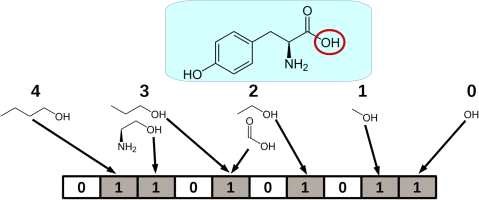
Molecular fingerprints are crucial tools in cheminformatics, as shown in Figure 1, representing molecular structures as binary or integer strings [2, 3, 4]. These strings capture the presence or absence of substructures or features within a molecule, enabling efficient comparison and analysis of chemical compounds. The Tanimoto coefficient is a widely used metric for measuring the similarity between two sets of molecular fingerprints [5]. It quantifies the degree of overlap between the fingerprints, providing a value between 0 and 1, where 1 indicates complete similarity. This coefficient is instrumental in various applications, such as virtual screening, clustering, and quantitative structure-activity relationship (QSAR) modeling, where assessing the similarity between molecules is essential [2].

Figure 1 Graphical representation of the Morgan fingerprint. The figure illustrates generating a molecular fingerprint using the Morgan algorithm. The fingerprint captures the substructural features of a molecule, enabling efficient comparison and similarity analysis between molecules [2].

1.3 Machine Learning, Artificial Neural Networks

Machine Learning (ML) is a field of computer science that focuses on imitating the way humans learn by using data and algorithms, aiming to create models that produce desired outputs for given inputs and progressively improve accuracy. Recently, generative artificial neural networks have been outperforming many previous approaches in terms of performance [4, 6].

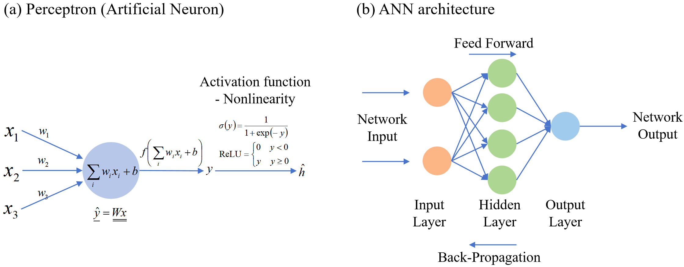
Artificial neural networks are machine learning models based on matrix mathematics that simulate the human nervous system as a simplified logical system. Artificial neural networks perform computations using the perceptron as the basic unit, as illustrated in Figure 2. This involves linear transformations of given input values through matrix operations, followed by the application of a nonlinear activation function to produce the output. Connecting multiple artificial neurons forms an artificial neural network, and when arranged in multiple layers, adding many hidden layers creates a Deep Neural Network. The goal of this process can be described as finding the weight matrix W that produces the desired results for a given situation through optimization operations such as gradient descent, based on mathematical principles [7].

Figure 2 Perceptron and simple ANN architecture [7].

Various neural network models are proposed depending on how artificial neurons are arranged to produce the desired output. Notable examples include Recurrent Neural Networks (RNNs) and Convolutional Neural Networks (CNNs).

Recurrent Neural Network (RNN) is structured to process sequential data by receiving outputs from previous stages as part of the input for the current stage, as illustrated in Figure 3. This model is commonly used for processing sequential data such as time series measurements or natural language [7].

Figure 3 Simple diagram of a recurrent neural network [7].

However, simple RNNs suffer from the gradient vanishing problem (long-term dependency), where the gradient value becomes close to zero as the layers deepen, rendering it meaningless during gradient computation for parameter determination. To address this, Long Short-Term Memory (LSTM) [8] was proposed. Nonetheless, LSTM's complex structure requires a large number of parameters, which can lead to overfitting if data is insufficient. To mitigate this, a Gated Recurrent Unit (GRU) [9] was proposed. This study utilized GRU to process sequential data like SMILES.

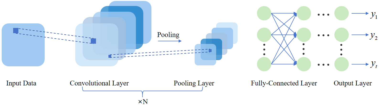
Convolutional Neural Network (CNN) is a model that creates maps through convolutional layers and dot product operations (convolution operations) with structured input data, as shown in Figure 4. It is primarily used to obtain features from grid-like data such as image processing [10]. This study employed CNN for analyzing NMR spectrum information.

Figure 4 A simple schematic diagram of convolutional neural network [7].

Error is defined as the loss function, which serves as the objective function. This can be formalized through mathematical development to establish the theoretical basis. Various loss functions exist; in this study, Mean Squared Error (MSE) and Cross Entropy were used. MSE is the average of the squared differences between the true values and the predicted values. It is represented as follows: (the $i^{\text{th}}$ true value: $y_i$, predicted value by the model ${\hat{y}}_i$)

Cross entropy measures the distance between the actual distribution and the distribution predicted by the model, and is represented as follows:

1.4 NMR Spectroscopy

Nuclear Magnetic Resonance (NMR) spectroscopy is a powerful analytical technique used to determine the content, purity, and molecular structure of a sample. By exploiting the magnetic properties of certain atomic nuclei, NMR provides detailed information about the arrangement of atoms within a molecule. This technique is widely employed in chemistry, biochemistry, and medicine for structural elucidation, compound identification, and studying molecular dynamics. NMR spectroscopy offers unparalleled insights into molecular structures, making it indispensable in research and quality control.

1.5 Previous Studies on Computational Tools for NMR Analysis

Numerous studies have focused on developing and enhancing computational tools for NMR analysis [11, 12], aiming to improve the accuracy and efficiency of molecular structure predictions from NMR data [4]. These tools leverage advances in machine learning, artificial intelligence [13], and cheminformatics to automate and refine the interpretation of NMR spectra [14]. By integrating computational methods with NMR spectroscopy, as shown in Figure 5, researchers have achieved significant strides in resolving complex molecular structures, identifying unknown compounds, and accelerating the analysis process [15, 16]. Recent advances in transformer models have demonstrated significant potential for NMR spectral analysis [22]. Automated frameworks for NMR spectral analysis, such as those proposed by [23], have shown promise in improving the efficiency of structure elucidation. Automated frameworks for NMR spectral analysis, such as those proposed by [23], have shown promise in improving the efficiency of structure elucidation. The continuous evolution of these computational tools promises to further advance the capabilities of NMR spectroscopy, enhancing its application in various scientific fields [17, 16].

Figure 5 The Spec2Mol model translates mass spectrometry (MS/MS) spectra into molecular structures using deep learning. The figure illustrates the integration of spectral data and molecular generation in the model [19].

2.1 SMILES

The Simplified Molecular-Input Line-Entry System (SMILES) data serves as a standardized method for representing chemical structures, which is pivotal for computational analysis. SMILES notations translate the graphical representations of molecules into text strings, enabling seamless input and manipulation of chemical data within various software environments. This standardization facilitates the efficient storage, retrieval, and comparison of molecular structures across diverse chemical databases and computational platforms. By providing a concise and unambiguous description of molecular entities, SMILES data allows for streamlined integration into cheminformatics workflows, aiding in tasks such as virtual screening, molecular modeling, and predictive analytics. The utility of SMILES extends to various applications in drug discovery, materials science, and chemical informatics, where accurate and standardized chemical representations are crucial for computational tasks as shown in Figure 6.

Figure 6 Example of SMILES strings from PubChem's CID-SMILES file.

2.2 NMR

NP-MRD (Natural Products Magnetic Resonance Database) is crucial for accurately predicting molecular structures[21]. It captures the interaction of atomic nuclei with magnetic fields, providing detailed insights into atom composition and arrangement. This information is used to identify molecular structures, elucidate complex organic compounds, and verify chemical syntheses. NMR data includes parameters like chemical shifts, coupling constants, and signal intensities, which contribute to the structural determination process. By analyzing these spectral features, chemists can deduce the connectivity, stereochemistry, and dynamic behavior of molecules [18]. The integration of NMR data with computational tools enhances the accuracy and efficiency of structure prediction, making it valuable in fields like organic chemistry, biochemistry, and pharmaceuticals. Combining NMR data with machine learning and other computational methods further enhances structural prediction capabilities.

2.3 Model Architecture

When analyzing NMR spectra, the thought process can be broadly divided into two steps:

Obtaining Valid Information from the Spectrum. This involves gathering information such as peak positions, integrals, and splitting patterns to infer details about functional groups and adjacent structures of the target molecule.

Inferring a Rational Molecular Structure Based on the Information. Using the obtained information to hypothesize the molecular structure. To represent this process of deriving the target molecule, the model is proposed with three main components:

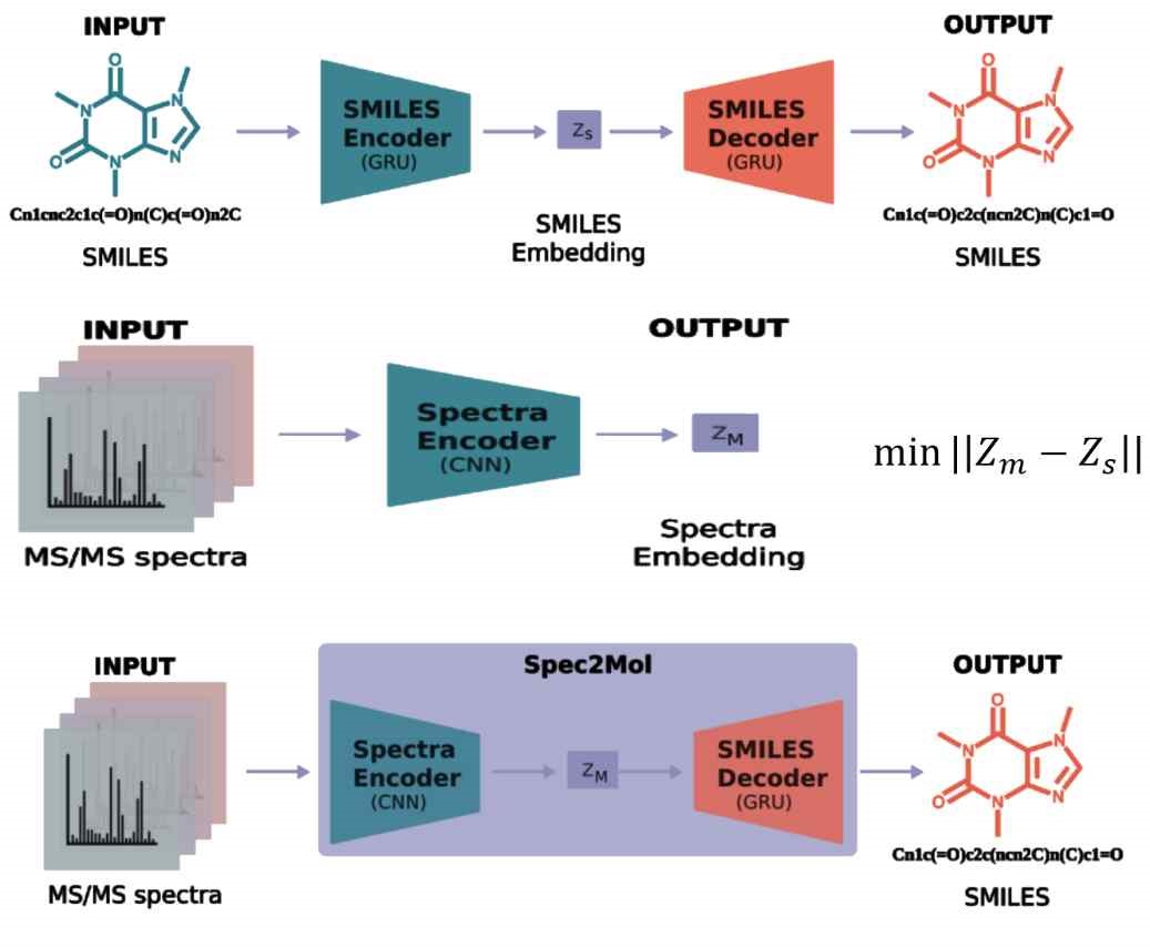
The SMILES encoder and decoder can be combined to form an SMILES autoencoder, which can then be used to train the NMR encoder with the obtained latent vectors. Ultimately, connecting the NMR encoder and SMILES decoder completes the model architecture for inferring the target molecule from NMR spectra, as shown in Figure 7.

Figure 7 Architecture of the proposed model (NMRGen).

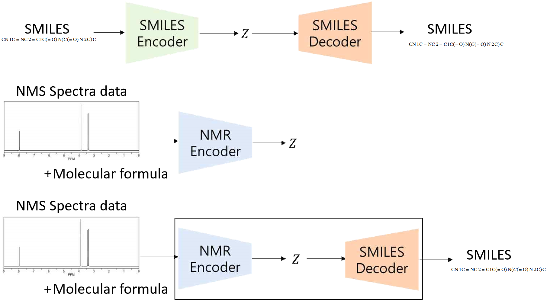
The model consists of three main components: the SMILES encoder, the SMILES decoder, and the NMR encoder. The SMILES encoder compresses SMILES strings into latent vectors, while the NMR encoder processes NMR spectra and molecular formulas to produce similar latent vectors. The SMILES decoder reconstructs SMILES strings from the latent vectors. The final model connects the NMR encoder and SMILES decoder to predict molecular structures from NMR spectra.

2.4 SMILES Encoder and Decoder

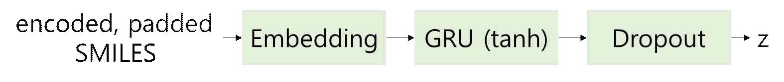
SMILES consist of sequential information. To create a model for analyzing this, the study utilized GRU, an improved version of RNN. The SMILES encoder and decoder were constructed using embedding, dropout, and linear layers, as shown in the Figure 8.

Figure 8 Architecture of the SMILES encoder and decoder. (a)The encoder employs embedding, GRU layers, and linear transformations to convert SMILES strings into latent vectors, capturing their syntax and structure. (b)The decoder reconstructs SMILES strings from latent vectors using GRU layers and linear transformations, generating probability distributions to form valid molecular structures.

2.5 NMR Encoder

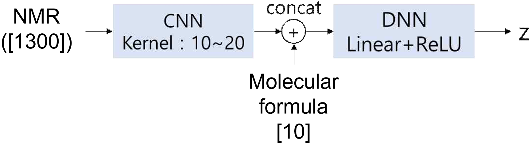
The NMR encoder was constructed using CNN and DNN (Linear layer + ReLU activation function). The CNN is designed to extract spectral features, such as peak splitting patterns, from NMR spectra, mimicking the human ability to interpret complex spectral data, with the number of kernels corresponding to the typical number of distinguished splitting types, as shown in Figure 9. In this case, the size of z is the same as that for the SMILES encoder and decoder.

Figure 9 NMR encoder processes NMR spectra and molecular formulas using convolutional neural networks (CNNs) and dense neural networks (DNNs). The CNN extracts features from the spectra, while the DNN maps these features to latent vectors that match those produced by the SMILES encoder.

2.6 Training Process

The training process is divided into three stages, conducted in the sequence of Train 1, Train 2, or Train 0, 1, 2 as follows:

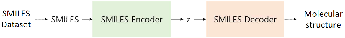
Training the SMILES Autoencoder. Train 1 involves training the SMILES autoencoder using the SMILES dataset. In this stage, the SMILES encoder and decoder are connected to predict the probability of each character at every position from the input SMILES data as shown in Figure 10. The training aims to minimize the Cross-Entropy between the predicted characters and the original SMILES data.

Figure 10 Training of SMILES encoder and decoder.

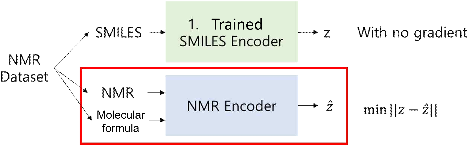
Training the NMR Encoder. Train 2 focuses on training the NMR encoder with the NMR dataset. For each molecule, the SMILES string is passed through the SMILES encoder (trained in Train 1) to obtain a latent vector. Concurrently, the NMR spectra and molecular formula are processed through the NMR encoder to produce another latent vector. Training is performed to minimize the Mean Square Error between these two latent vectors. The SMILES encoder parameters are fixed during this training in Figure 11.

Figure 11 Training of NMR encoder. The NMR encoder is trained to produce latent vectors that match those generated by the SMILES encoder. The mean squared error (MSE) between the latent vectors from the SMILES encoder and NMR encoder is minimized during training.

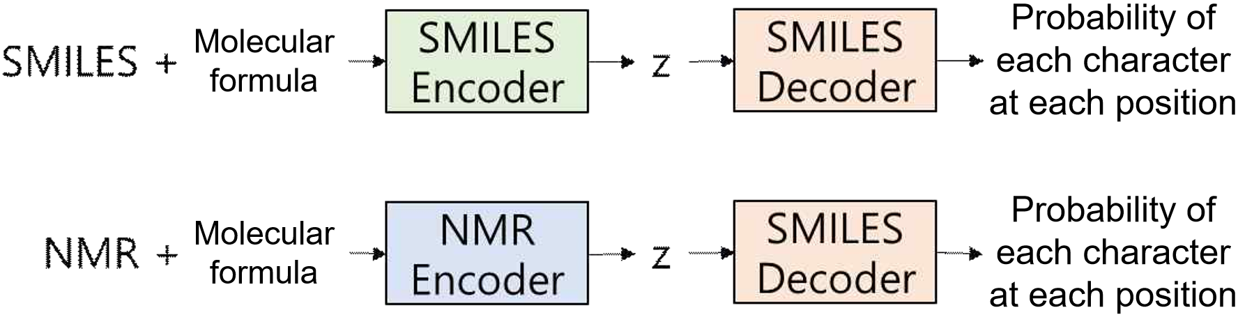
Simultaneous Training of SMILES Encoder, Decoder, and NMR Encoder. In addition to the above processes, Train 0 was introduced to enhance the overall training effect and incorporate NMR data into the latent vector representation [20]. In this process, all three models—the SMILES encoder, SMILES decoder, and NMR encoder—are trained simultaneously. Training proceeds in the sequence of Train 0, 1, 2. The combined Cross Entropy loss of the SMILES encoder-decoder and NMR encoder-decoder models is used to update the parameters of all three models in Figure 12.

Figure 12 Simultaneous training of SMILES encoder, decoder, and NMR encoder.

2.7 Testing Process

The trained NMR encoder and SMILES decoder are connected to create a model that generates SMILES strings from NMR spectral information. The final test loss is evaluated by measuring the Cross-Entropy between the true SMILES strings and the generated strings, assessing the accuracy of the model, as shown in Figure 13.

Figure 13 The final model for generating SMILES from NMR spectra.

Figure 14 Training and validation loss history for latent vector size [B, L*F].

3.1 Latent Vector Variations

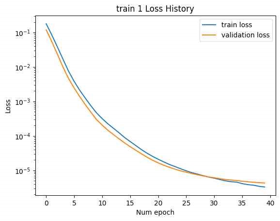
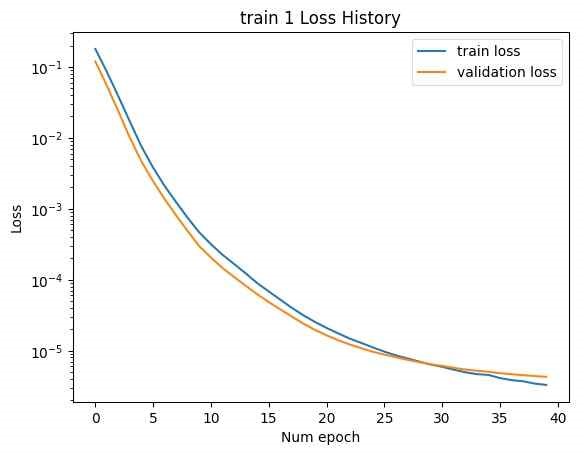
In the initial attempt, the entire GRU output of the SMILES encoder, with a tensor size of [B, L*F], was used as the latent vector, as shown in Figure 14. (The NMR encoder had 15 CNN kernels, 4 DNN layers, and a hidden dimension of 10,000.) Training was conducted with two datasets: train 1 and train 2. The loss history for epochs is shown below. (Minimum validation loss for train 1: $4.267\times {10}^{-6}$, $4.267\times {10}^{-6}$, minimum validation loss for train 2: 0.2285.)

Although the loss for each training session was relatively low, excessive training time was encountered due to the large number of model parameters, leading to premature termination of the training process before convergence.

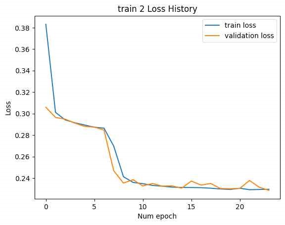
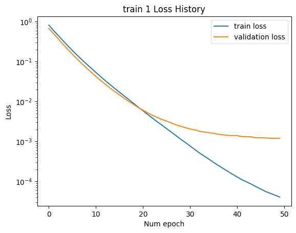
In Figure 15, to address this, linear layers with dimensions LF to F and F to LF were added at the beginning and end of the SMILES encoder and decoder, respectively. This adjustment modified the latent vector size to [B, F]. The number of CNN kernels in the NMR encoder was reduced to 10, and the number of DNN layers was reduced to 3. The training was then conducted with Train 1 and Train 2. The loss history concerning epochs is shown below. (Minimum validation loss for train 1: 0.004206, minimum validation loss for train 2: 20.49.)

Figure 15 Training and validation loss history for latent vector size [B, F].

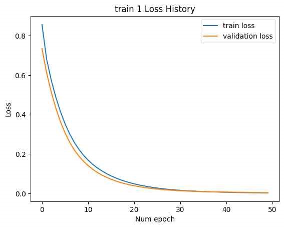
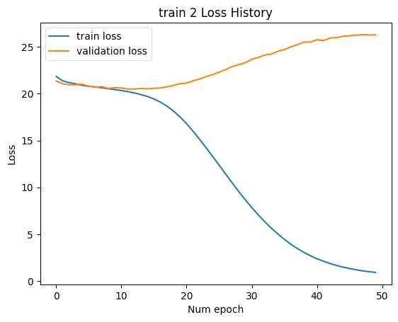
In this case, while the training loss decreased, the validation loss increased, indicating an overfitting issue. In Figure 16, address overfitting, the latent vector size was increased to [B, 2F], and the experiment was repeated. (Minimum validation loss for train 1: 0.001193, minimum validation loss for train 2: 16.04.)

Figure 16 Training and validation loss history for latent vector size [B, 2F].

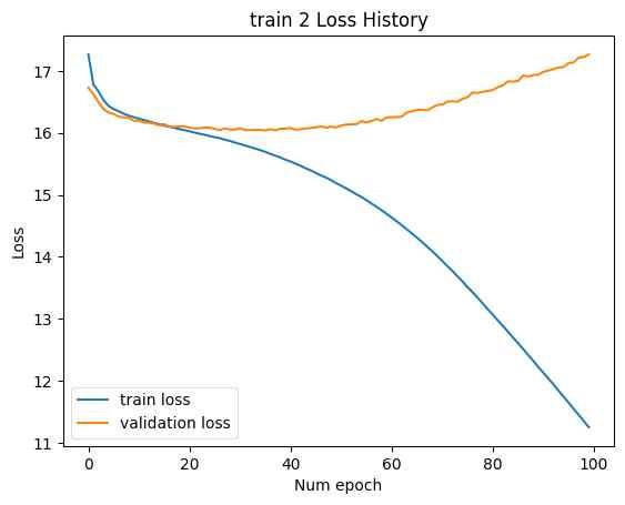
Increasing the latent vector size resulted in reduced minimum validation loss for both trains. However, overfitting was still observed in train 2. Despite this, increasing the latent vector size led to a decrease in final test loss and produced a more varied set of SMILES, although valid SMILES were not found in the cases where the latent vector size was [B, L*F] and the training was halted.

3.2 Comparison of Train Processes

A comparison of the final test losses between experiments using trains 0, 1, and 2 and those using only trains 1 and 2 showed no significant differences. However, a noticeable difference was observed between cases where only train 0 was performed versus where all trains 0, 1, and 2 were performed. The latter achieved a lower final test loss.

3.3 Hyperparameter Variations

To improve learning, various hyperparameters were adjusted while keeping the latent vector size fixed at [B, F]. Changes were made to learning rates, learning rate schedulers and annealing, hidden dimensions and layers, and weight decay, among other factors. No significant changes were observed. The loss history from the experiment with the smallest final test loss is shown below.

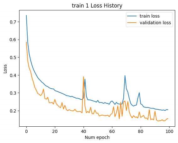
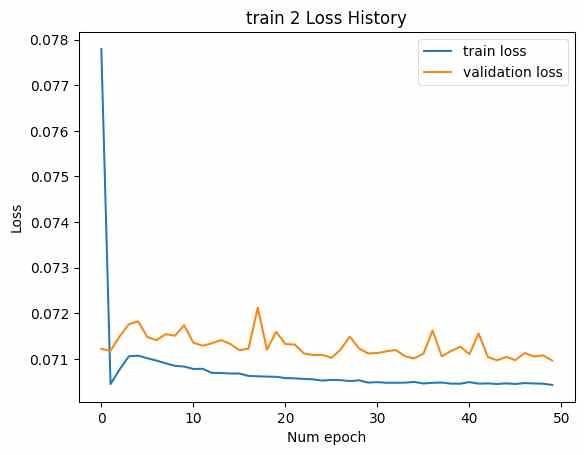
(Train 1, 2: Best validation loss for train 1: 0.1416, best validation loss for train 2: 0.0710, final test loss: 1.273, valid SMILES: 0)

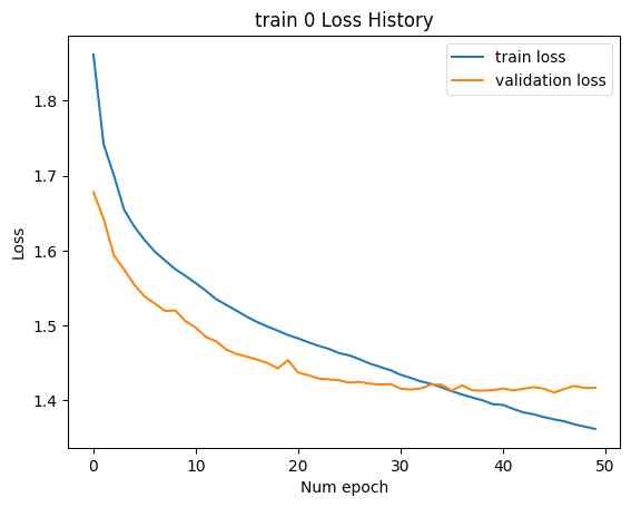
(Train 0, 1, 2: Best validation loss for train 0: 1.4104, best validation loss for train 1: 0.1411, best validation loss for train 2: 0.0682, final test loss: 1.282, valid SMILES: 2, as shown in Figures 17 and 18).

Figure 17 Loss history for the experiment with the smallest final test loss (Trains 1 and 2).

Figure 18 Loss history with the smallest final test loss for Trains 0 and 1.

3.4 Valid SMILES

Throughout the experiments, valid SMILES that conform to SMILES syntax were rarely generated. The valid SMILES that were produced mostly took the form of CCC…C, which is less likely to be grammatically incorrect, as shown in Figure 19.

Figure 19 Example of Generated Valid SMILES: Molecule with CCC…C Structure.

In Table 1, to assess the similarity between the generated valid SMILES and the correct molecules, the Tanimoto coefficient was used. On average, the coefficient values ranged between 0.1 and 0.2. This indicates that the generated valid SMILES were not similar to the actual target molecules.