


IECE Transactions on Emerging Topics in Artificial Intelligence
ISSN: 3066-1676 (Online) | ISSN: 3066-1668 (Print)
Email: [email protected]

In recent years, there has been a growing global emphasis on sustainable and renewable energy, driven by concerns over climate change and the finite nature of fossil fuels. Renewable electricity, a key component of the energy transition, continues to increase its share in global power generation. As this transition unfolds, precise forecasting of renewable energy demand becomes essential. Accurate prediction of electricity demand is crucial in today's society, as it not only supports the achievement of sustainable energy development goals but also provides valuable insights for the transformation of electricity markets and the future of energy needs [1, 2]. By combining precise forecasts of electricity demand with renewable energy supply, new decision-making strategies can be proposed for global system planning. Therefore, developing an effective electricity demand forecasting framework is imperative.
In traditional electricity consumption forecasting methods, regression analysis and time series models are the most commonly used techniques. Bianco et al. [3] applied linear regression models to predict electricity consumption in Italy, while Arisoy et al. [4] used historical time series data to forecast residential electricity demand. Several other studies [5, 6, 7] employed ARIMA models and seasonal ARIMA models to predict electricity loads. Mitkov et al. [8] developed prediction models for future energy demand using ARIMA models based on the linear characteristics of historical electricity consumption data. However, econometric models tend to perform poorly in predicting nonlinear sequences due to their complexity [9]. Amjady et al. [10] proposed an enhanced ARIMA model for short-term electric load forecasting, which incorporates both temperature and electric load data to predict hourly loads and daily peak electricity demand. Feinberg et al. [11] integrated temporal factors, weather data, and customer segmentation in their short-term electric load forecasts. Despite these advances, linear regression models face significant challenges in capturing nonlinear relationships, especially when the demand for electricity and its influencing factors exhibit nonlinear dynamics. This makes it difficult for linear regression models to accurately capture nonlinear load demand patterns across different time periods [12].
With the advancement of artificial neural networks, the ability to address nonlinear problems has significantly improved [13, 14]. This improvement allows solutions to overcome the limitations of linear regression models in handling nonlinear relationships [15, 16]. As a result, some researchers have started combining regression models with artificial intelligence in demand forecasting [17]. For instance, Valenzuela et al. [18] integrated the nonlinear mapping capability of artificial neural networks with time series models, proposing an ARIMA-ANN model. In this approach, a fuzzy logic expert system was used to determine the differencing order of the ARIMA model, as well as the orders of the autoregressive (AR) and moving average (MA) components. Fan et al. [19] applied ARIMA to filter the linear trend in time series data and used the residuals as input to an LSTM model, developing an ARIMA-LSTM ensemble model to predict oil well production effectively. Nie et al. [20] introduced a novel hybrid model combining data preprocessing, individual forecasting algorithms, and weight determination techniques, demonstrating higher accuracy and improved forecasting performance. However, renewable energy power systems are complex and dynamic, influenced by various factors such as weather, technological advancements, policy changes, and social trends [21]. These models may struggle when dealing with non-time-series electricity demand data, suggesting the need for further research into more advanced predictive models.
Multimodal information fusion refers to the process of collecting and integrating information from diverse data sources to improve decision-making, forecasting, recognition, or classification tasks [22], [23]. Recently, an increasing number of scholars have focused on applying multimodal fusion to electricity demand forecasting. For example, Xuan et al. [24] employed a feature selection algorithm based on random forests to identify key input features for load forecasting models. After selecting the input features, they proposed a hybrid neural network algorithm for short-term load forecasting, which leverages multimodal fusion. Ji et al. [25] developed an advanced multimodal fusion model with enhanced predictive performance by combining the outputs of three models—Gradient Boosting Decision Trees, Extreme Gradient Boosting, and Light Gradient Boosting Machine—through decision fusion. To capture more comprehensive temporal and spatial features from the original data, Kong et al. [26] proposed an integrated approach for short-term load forecasting, combining Empirical Mode Decomposition (EMD), the similar day method, and deep neural networks. Within this framework, a CNN-LSTM model based on EMD is used to extract multimodal spatiotemporal features. These multimodal fusion models not only increase the complexity and dimensionality of the forecasting models but also improve prediction accuracy and reliability by capturing a broader range of influencing factors. However, there is currently no literature on how to effectively select the modality that best represents key factors influencing power demand, such as weather conditions, economic activities, political events, and social behavior patterns.
Initially, we conduct an analysis of data relevant to short and long-term electricity demand. The data is categorized into short and long-term forecasting data. Subsequently, CNNs are employed to extract two types of latent features pertinent to the research objective from numerical time series data and textual data.
Regarding the fusion methodology, we adopt a concatenation fusion approach to organically merge the temporal latent features and textual latent features. The fused features are then fed into a model constructed using Bi-GRU for prediction.
Ultimately, the constructed short-term and long-term demand forecasting models are validated through experimentation, demonstrating their superior predictive performance compared to the ARIMA model, single GRU network, and combination model (EEMD-ARIMA).
Prediction refers to estimating future trends using existing data or past experiences. Renewable energy demand forecasting involves multiple influencing factors, including energy consumption patterns, policy changes, technological advancements, climate conditions, and economic growth. Its primary objective is to assist governments, energy enterprises, and market decision-makers in making scientifically sound plans, improving energy supply chain management efficiency, optimizing grid dispatching, and promoting sustainable energy development. Based on the forecasting time horizon, renewable energy demand forecasting can be categorized into short-term, medium-term, and long-term predictions.
(1) Short-term renewable energy demand forecasting typically covers a few days, weeks, or months into the future. It primarily relies on recent weather data, grid load conditions, and energy consumption patterns. It is widely used in power dispatching, demand response management, and short-term energy market transactions. For example, given the high variability of wind and solar energy, short-term forecasting helps grid operators efficiently allocate energy storage resources and optimize the balance between electricity supply and demand.
(2) Medium-term renewable energy demand forecasting involves predicting energy demand trends over the coming months to several years. Compared to short-term forecasting, medium-term prediction requires considering a broader range of factors, such as economic development, social changes, policy adjustments, and industrial structure upgrades. For instance, governments can utilize medium-term forecasting results to design renewable energy subsidy policies, optimize energy infrastructure construction, and facilitate sustainable energy transitions.
(3) Long-term renewable energy demand forecasting spans several years to decades and involves more complex factors, including technological progress, global climate change, energy market transformations, and carbon neutrality goals. Although long-term forecasting entails greater uncertainty and risks, it is crucial for formulating national energy strategies, investing in new energy projects, and establishing carbon reduction plans. For example, energy companies can use long-term predictions to plan the development and investment of wind and solar energy projects, aligning with future energy structure adjustments.
Traditional forecasting methods: In the research of electricity demand forecasting, traditional methods primarily rely on statistical analysis and time series modeling. Regression analysis is a common statistical approach; for instance, Bianco et al. [3] utilized a linear regression model to predict electricity consumption in Italy. Additionally, time series methods, such as ARIMA and its improved versions, have been widely applied in electricity load forecasting. For example, some employed ARIMA and seasonal ARIMA models [5, 6, 7] to forecast electricity load, respectively. Furthermore, Mitkov extended the use of the ARIMA model by incorporating the linear characteristics of historical electricity consumption data to establish an energy demand forecasting model [8]. However, traditional models often underperform when dealing with complex nonlinear features, especially when electricity demand is influenced by multiple factors such as weather, policy changes, and economic fluctuations. Statistical models frequently fail to accurately capture the intricate dynamic patterns in the data, leading to diminished forecasting performance [9].
Deep learning prediction methods: ANN with their powerful nonlinear modeling capabilities, can effectively address the limitations of traditional methods in handling complex data patterns [13]. For instance, Valenzuela et al. [18] proposed an ARIMA-ANN hybrid model that integrates a fuzzy logic expert system to optimize the parameters of the ARIMA model, thereby improving prediction accuracy. Additionally, Fan et al. [19] employed ARIMA to preprocess time series data and fed the residuals into an LSTM network, constructing an ARIMA-LSTM integrated forecasting model to enhance the accuracy of oil well production predictions. Nie et al. [20] utilized a multi-objective grey wolf optimization algorithm to combine radial basis function networks, generalized regression neural networks, and extreme learning machines, further improving prediction performance. These studies demonstrate that integrating traditional statistical methods with deep learning techniques can uncover trends in electricity demand from time series data, significantly enhance the accuracy of electricity demand forecasting, and improve adaptability to complex load variations. However, although combining regression models with deep learning models can effectively leverage the strengths of each approach to improve prediction accuracy, renewable energy power systems remain inherently complex and dynamic. These systems are influenced by multiple factors such as weather patterns, technological advancements, policy changes, and social trends, which are often difficult to fully capture using single time series data alone.
Multimodal fusion methods: Multimodal information fusion involves integrating data from various sources to improve decision-making [22], prediction [23], recognition, and classification tasks. In recent years, this approach has garnered increasing attention in electricity demand forecasting. For instance, Xuan et al. [24] employed a random forest-based feature selection algorithm to optimize input features for load forecasting models and proposed a hybrid neural network-based method for short-term load forecasting using multimodal fusion. Ji et al. [25] applied decision fusion by combining GBDT, XGBoost, and LightGBM to develop a multimodal fusion model with enhanced predictive performance. Furthermore, Kong et al. [26] introduced a short-term load forecasting method that integrates Empirical Mode Decomposition (EMD), the similar-day method, and deep neural networks. This study utilized an EMD-based CNN-LSTM approach to extract multimodal spatiotemporal features from the input data, improving prediction accuracy.
Despite significant progress in multimodal fusion research, several key challenges remain. For instance, effectively selecting key modalities to comprehensively represent core factors influencing electricity demand—such as weather conditions, economic activities, policy changes, and social behavior patterns—remains an unresolved issue. Additionally, traditional deep learning models still face limitations in handling long-sequence data, making it difficult to capture long-term dependencies fully. To address these challenges, this paper proposes a multimodal fusion-based forecasting model using CNN-Bi-LSTM. This model leverages CNN's feature extraction capabilities and Bi-LSTM's bidirectional learning ability in processing time-series data, enabling more efficient capture of spatiotemporal characteristics in electricity demand and enhancing prediction accuracy and stability.
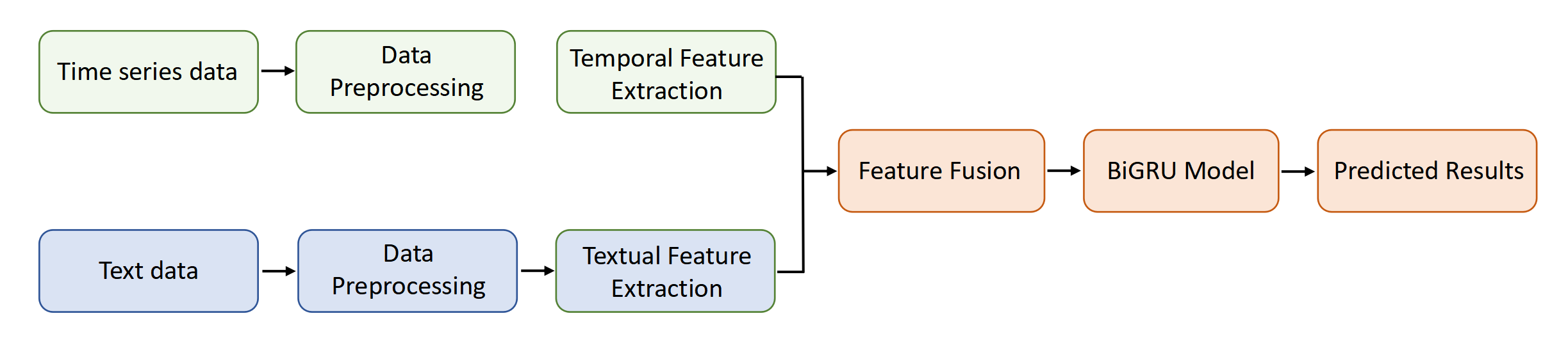
In order to combine the temporal information of time series data with the nature information of textual data, we propose a novel ensemble prediction modeling approach based on multimodal information fusion for quantitative analysis and forecasting of electricity demand and renewable energy supply. The fundamental principle of the prediction model lies in the concept of multimodal information fusion-driven modeling, where the complementary nature of time series data and textual data forms the foundational assumption for building effective models. The framework of this model is illustrated in Figure 1, consisting of four main steps:
(1) Data Preprocessing: The preprocessing of both modalities of data is conducted separately. Time series data is transformed into one-dimensional format using time window techniques, while textual data undergoes structured processing using the Word2Vec model, capable of extracting semantic features of text.
(2) Feature Extraction: Utilizing CNNs, we extract the hidden features of the processed time series and textual data, and then combine the features extracted from both data modalities as input for the prediction module.
(3) Feature Fusion: Considering the heterogeneity of the original data, this paper employs vector concatenation to merge and integrate the hidden features of the two modalities.
(4) Prediction Module: Model training is conducted using Bi-GRU, which exhibit favorable properties for processing sequential data.
It is worth noting that due to the differences between mid-term and long-term predictions in time series and textual data, this paper adopts the same model framework to train corresponding mid-to-long-term electricity demand prediction models using different time series and textual data.
In most cases, the raw data we acquire tends to be messy and incomplete, making it challenging for machine learning models to extract meaningful information. To ensure that the data fed into the input feature extraction module meets the requirements, some preprocessing of the raw data is necessary.
Time series data preprocessing: Our process begins with an initial cleanup of the raw time series data, starting with the filling of missing values to ensure data completeness and continuity. This step is crucial for maintaining data quality and for subsequent analyses. Following this, we employ the sliding window technique for further processing. The sliding window technique moves a fixed-length window across the time series, extracting segments of data from each window. This transforms continuous data segments into a series of independent observations, making the processed data more suitable for input into CNN. This approach not only aids in capturing local features and trends within the time series data but also facilitates the model's learning of temporal dependencies, laying the groundwork for subsequent deep learning model training and prediction. Finally, to map the data within a fixed range, we utilize the method of min-max normalization to process the input data. The min-max normalization formula is expressed as follows:

Textual data preprocessing: The raw textual data is considered unstructured data and requires data preprocessing before feature extraction. During the process of converting text data, it's essential to preserve as much useful information as possible. Basic preprocessing of textual data includes steps like tokenization and stop word removal. Subsequently, the Word2Vec model [27] is utilized for text representation, also known as text vectorization (Word Embedding). This technique enables quantitative measurement of the relationships between words, facilitating the exploration of connections between them. Text vectorization eliminates the cumbersome task of feature processing, maximally preserving the essential content within the text. The model's network structure comprises three layers: the input layer, the projection layer, and the output layer, as illustrated in Figure 2. The purpose of training this model is to maximize the value expressed as follows:
where represents the window size, and the conditional probability is designed as:
However, Word2Vec has limitations, such as its inability to fully capture contextual nuances and polysemy in textual data. To address this, alternative or complementary methods such as Bidirectional Encoder Representations from Transformers (BERT) or GloVe could be explored to enhance the representation of textual information and mitigate potential biases.
This section focuses on exploring how to perform feature extraction from preprocessed data, a key aspect of the method proposed in this paper. The input data consists of two distinct datasets, comprising time series data and related textual data. We aim to extract data features from these two types of data that are suitable for constructing a Bi-GRU prediction model.
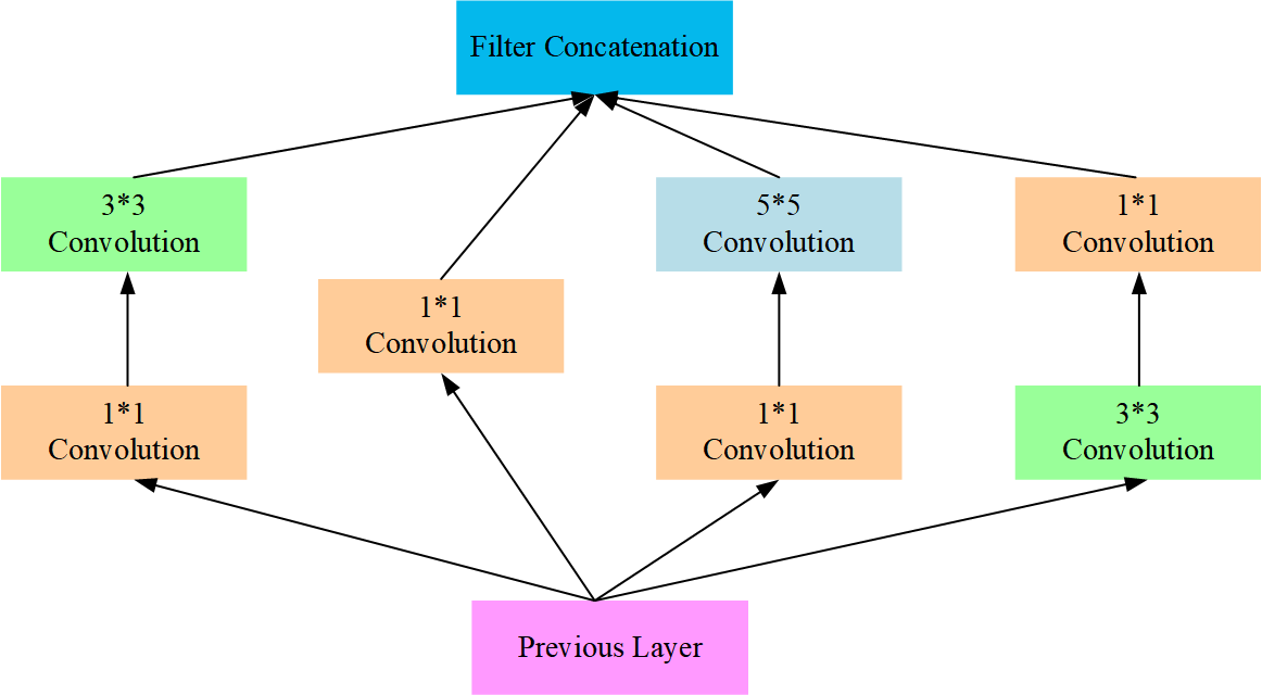
Feature extraction of time series data: The Inception architecture is an innovative convolutional neural network design aimed at capturing multi-scale image features by paralleling convolutions of varying sizes, while employing convolutions for dimensionality reduction to enhance computational efficiency and minimize overfitting [28], as depicted in Figure 3. This architecture has undergone several iterations, incorporating optimizations such as batch normalization and residual connections, showcasing exceptional performance and efficient computation in tasks like image recognition and classification. The entire process of using CNNs to extract features from time series data is outlined as follows:
First, the convolutional layer extracts features from the input data.
where , , denote the convolution kernel parameters.
Second, in order to accelerate the convergence speed, the ReLU function is added as an activation function after the convolutional layer. The formula is as follows:
Third, after the convolutional layer, a pooling layer is introduced to reduce the dimensionality of the feature maps and prevent the curse of dimensionality. The max-pooling strategy is applied to perform pooling operations on the feature maps obtained after the convolution operation, effectively reducing the number of parameters in the model while retaining useful information. This pooling operation is a common technique used to reduce the complexity of computations and improve the performance of the model by reducing the dimensionality of the input feature maps. The formula is as follows:
where represents the feature map.
Finally, add a flattening layer to flatten the pooled feature maps into one-dimensional form, forming the final latent feature for the time series data.
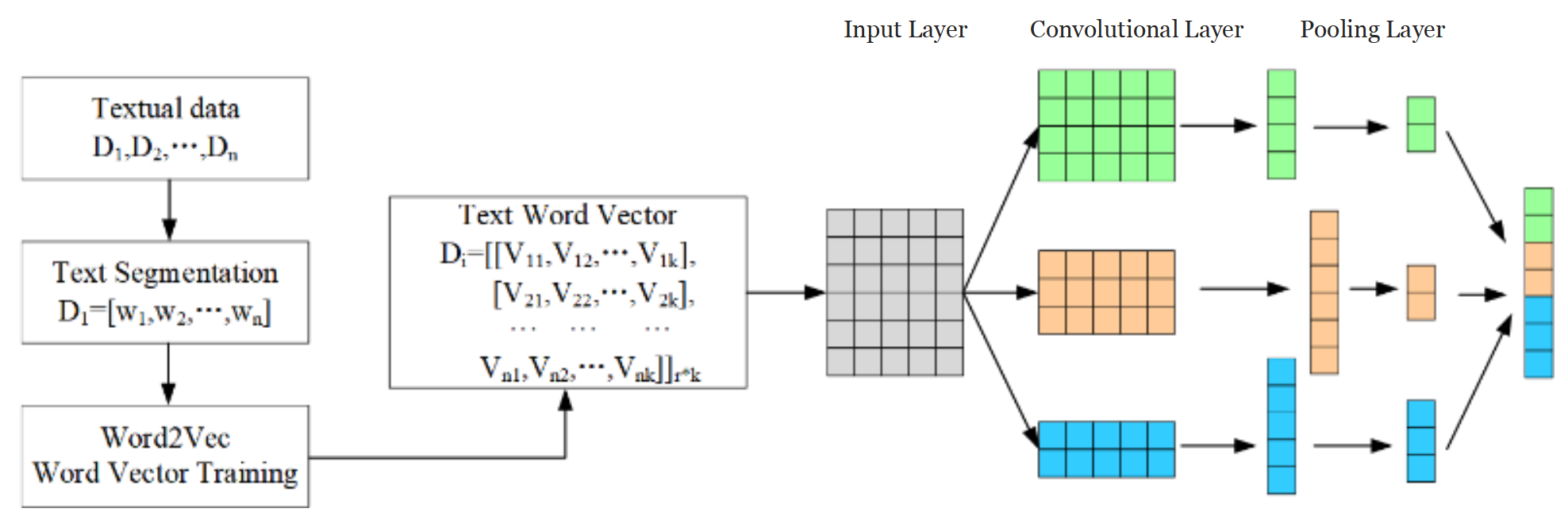
Text data feature extraction: Traditional text feature extraction methods face challenges with high dimensionality and inefficiency. This study adopts a CNN-based approach proposed by Er et al. [29], which not only excels in feature extraction but also aligns structurally with previously extracted time series features. The text feature extraction process, illustrated in Figure 4, utilizes convolution and pooling as core mechanisms. These operations process fixed-length text sequences to distill primary features, which are then transformed into advanced features through further convolution and pooling. After being processed by a flattening layer, these features are directly output as the text features (TF) required for this study.
The Inception structure in CNNs is particularly effective for text feature extraction due to its multi-scale processing capability, allowing simultaneous capture of both local and global textual patterns. Its efficient architecture facilitates deep, complex feature learning without substantial computational cost, offering adaptability for various text analysis tasks while also mitigating overfitting through its parallel convolutional paths. This makes it adept at handling the intricacies of textual data, enhancing model performance across a range of linguistic analysis applications.
This paper adopts the feature-level fusion strategy to build the prediction model, merging the latent features obtained from the two modalities through multimodal fusion methods. For feature fusion, we choose the direct concatenation of feature vectors to preserve the original data information as much as possible. In the linear fusion method based on manual rules, weight values need to be manually set to adjust the proportion of feature vectors, which may introduce subjectivity and limitations. The similarity matrix approach requires computing the similarity matrix between feature vectors, which may encounter complexity issues in matrix calculations. On the other hand, the direct concatenation of feature vectors is relatively simple and straightforward, as it only involves concatenating the feature vectors together. Especially in the case of heterogeneous data, the direct concatenation method does not require additional calculations and transformations, making it more convenient and efficient. In summary, when performing feature fusion, the most suitable fusion method should be selected based on the specific situation to maximize the extraction and preservation of data information.
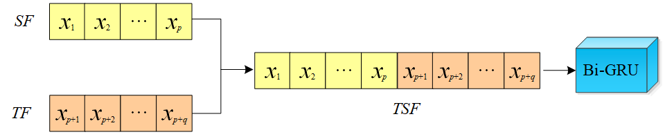
Vector concatenation, or concatenation fusion as described by Yang et al. [30], involves joining latent features from time series and text data end-to-end for feature fusion, depicted in Figure 5. SF and TF denote latent features from time series and text, with elements like being vectors . This process leverages DenseNet's [31] concatenate operation to merge and aggregate flattened vectors post-extraction.
In this study, vector concatenation is adopted as the fusion method for textual and time series data, primarily due to its computational efficiency, interpretability, and suitability for electricity demand forecasting. Electricity demand forecasting involves time series data (such as historical load and meteorological factors) and textual data (such as policy announcements and news reports), which have distinct feature representations. Directly mapping them into the same space may result in information loss or distribution mismatches. Vector concatenation enables efficient information fusion while preserving the independent characteristics of each modality, avoiding the computational overhead and noise that more complex models might introduce. Moreover, electricity demand forecasting often requires high real-time performance, and vector concatenation offers a low computational cost, making it suitable for large-scale data processing and online prediction scenarios. Experimental comparisons demonstrate that this method achieves a good balance between prediction accuracy and computational efficiency in the fusion of time series and textual data, effectively meeting the practical application needs of electricity demand forecasting.
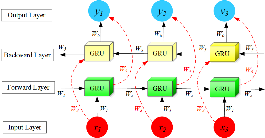
The prediction module employs the Bi-directional Gated Recurrent Unit (Bi-GRU) neural network (as shown in Figure 6), using the fused features TSF as input. Bi-GRU is chosen for two key reasons: First, its bidirectional processing effectively models temporal dependencies and mitigates the vanishing gradient problem. Second, while CNNs excel at extracting local features, Bi-GRU's long-term memory capability complements this by capturing broader temporal relationships.
Unlike traditional RNNs, Bi-GRU processes sequences in both forward and backward directions, allowing it to incorporate past and future context. Its architecture consists of input layers, bidirectional GRU layers, and output layers, where each GRU layer contains two subunits processing data in opposite directions. This enables the model to better understand sequential patterns. Bi-GRU has proven effective in tasks such as natural language processing, speech recognition, and time series analysis due to its ability to capture long-range dependencies efficiently.
First, for every GRU, the update gate decides how much of the past information should be retained for the current time step. It takes as input the concatenation of the previous hidden state and the current input . This gate determines the proportion of the previous hidden state that will be combined with the candidate hidden state . It is calculated using a sigmoid activation function as follows:
The reset gate controls how much of the past information should influence the calculation of the candidate hidden state . It also takes the concatenation of the previous hidden state and the current input as input and is computed using a sigmoid activation function as follows:
The candidate hidden state is an intermediate representation computed based on the reset gate and the concatenation of the modified previous hidden state and the current input . This candidate hidden state captures the potential new information for the current time step.
Finally, the update gate . decides how much of the candidate hidden state should replace the previous hidden state .
where denotes element-wise multiplication.
For Bi-GRU, the input sequence is , where is the -th element in the sequence. The goal of Bi-GRU is to model the entire sequence and extract bidirectional information from it. Bi-GRU consists of two independent GRUs: one for processing the forward sequence and the other for processing the backward sequence. For the forward GRU , the forward update gate determines how much the previous hidden state and the current input influence the current hidden state . It is calculated using a sigmoid function. Forward Reset Gate , the forward reset gate determines how much the previous hidden state and the current input influence the calculation of the candidate hidden state . Similarly, it is computed using a sigmoid function.
Finally, Bi-GRU concatenates the forward and backward hidden states to form the complete bidirectional context information. During training, Bi-GRU learns how to simultaneously consider both forward and backward information and generate the final sequential representation.
o assess predictive performance, the Root Mean Square Error (RMSE) and Mean Absolute Percentage Error (MAPE) are utilized to evaluate prediction accuracy. Additionally, the directional accuracy is evaluated using the Dstat metric. The calculation methods for these three metrics are as follows:
RMSE:
where is the total number of observations, represents the actual value, and denotes the predicted value.
MAPE:
where is the total number of observations, represents the actual value, and denotes the predicted value.
Dstat:
where is the total number of observations, represents the actual value at time , denotes the predicted value at time , and is the sign function. Indeed, smaller values of RMSE and MAPE indicate higher accuracy in horizontal predictions, indicating better performance of the prediction model. Conversely, a larger value of Dstat indicates better directional prediction accuracy.
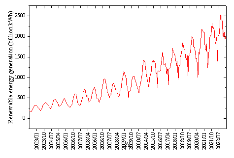
The predictive model requires heterogeneous data from multiple sources, including time series data and various types of textual data. In this study, datasets related to renewable energy supply time series data and relevant textual data were obtained. Each observation in the time series data is influenced by past observations, allowing for the prediction of future trends using its memory. For the renewable energy supply time series dataset, data were sourced from the official website of the National Bureau of Statistics. This dataset includes the electricity generation from major clean energy sources such as hydropower, wind power, and photovoltaic power, aggregated to monthly renewable energy supply. It covers 240 monthly observations from January 2003 to December 2022. As shown in Figure 7, with China actively promoting carbon peaking and carbon neutrality goals, and actively promoting the development of renewable energy, the country's renewable energy generation has been steadily increasing. Additionally, similar to electricity consumption, seasonal fluctuations are observed due to differences in power demand between seasons. Furthermore, due to China's energy resource endowment, the country's power supply is dominated by coal-fired power generation, and investment in renewable energy power generation is also constrained by existing large-scale coal-fired power installations, leading to a gradual slowdown in its growth rate.
The text data reveals that the demand for electricity is influenced by various factors, including political, economic, social, and technological aspects. Short-term electricity demand is primarily affected by seasonality, weather conditions, holidays, and special events, while medium and long-term forecasts place more emphasis on macroeconomic trends, population growth, energy policies, technological advancements, and societal changes. Therefore, different approaches may be required for short-term and long-term predictions based on text data. To ensure data accuracy, we collected official data concurrent with the electricity time series data through various means. Ultimately, the text dataset related to electricity demand covers 11342 records from January 2000 to December 2022.
The experiments in this article were conducted on the Keras deep learning framework. After preprocessing the input data, which includes time series and textual information, it was fed into the proposed CNN-Bi-GRU model for training.
For time series data, the first step involves filling in missing values within the dataset. Next, the time series data needs to be reshaped into one-dimensional format. A parameter, , is set to determine the size of the time window. The dataset is then structured such that the input samples for the time series data have a length of the preceding periods, and the value for the next period is used as the label. Subsequently, the data undergoes normalization using the min-max scaling method to map it within a fixed range. Finally, the dataset is divided into training and testing sets in a 9:1 ratio.
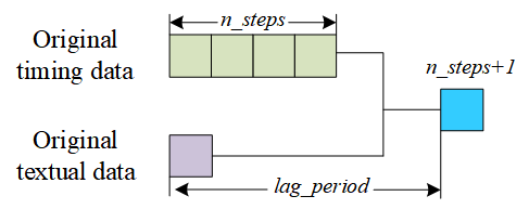
Before formally constructing the text data processing module, it is necessary to build the Word2Vec model for Chinese electricity demand. Firstly, each category of text data is aggregated on a monthly basis. Subsequently, textual data from different categories will be combined in chronological order, forming a corpus comprising all text data. Subsequently, this corpus is utilized to train the Word2Vec model, which will serve as the corpus for text vectorization in subsequent steps. Through multiple experimental comparisons, the dimensionality parameter value for vectors is set to 200, and the sliding window parameter value is selected as 15. Additionally, a lag_period is set as the text's lagging period to solve the delayed effect of text data. The corresponding labels are illustrated in Figure 8.
Upon formally constructing the text data processing module, after the basic preprocessing steps such as tokenization and stop word removal, the raw unstructured text data is vectorized using the pre-trained Word2Vec model. Subsequently, the parameter lag_period is set, and in conjunction with the pre-allocated training and testing datasets for the time series data, the training and testing datasets for the text data are partitioned. Finally, a subset of text data with a length of lag_period is retained for predicting future trends. Once the complete dataset is constructed, text data of length lag_period is retained based on the varying lag periods. For experiments, the ratio of the dataset to the training set is 9:1. The model is trained using the training set data and its predictive ability is evaluated using the validation set.
Subsequently, when constructing the temporal CNN neural network, the network is set up according to the Inception structure with adjustable width. For each channel of the network, an input layer, convolutional layer, pooling layer, and flattening layer are added, with the number of convolutional kernels in the convolutional layer set as an adjustable parameter. The outputs of the flattening layers from each channel are then aggregated to form the output of the temporal CNN neural network. As for the text CNN neural network, the operations are similar to the temporal CNN, except that an Embedding layer is added at the input layer to pre-train word vectors.
Finally, the Bi-GRU prediction module is constructed. The two types of latent features obtained from the feature extraction module are aggregated as inputs to the Bi-GRU neural network. The number of hidden neurons in the network is set as an adjustable parameter. MSE is utilized as the loss function, and Adam is employed as the optimizer to train the model.
The dataset is labeled using the renewable energy generation data from the previous 6 months and aggregated textual data from 36 months ago to predict the data for the next month. The final dataset comprises 234 entries, with 210 entries in the training set and 24 entries in the test set. This section will compare the effectiveness of the proposed renewable energy supply prediction model based on multimodal information fusion with ARIMA model, single GRU network, and composite model EEMD-ARIMA to validate its efficacy. This experiment is primarily divided into two parts: the first part focuses on short-term forecasting by month, while the second part deals with long-term forecasting on a semi-annual basis.
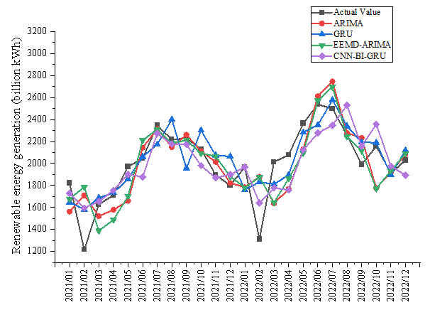
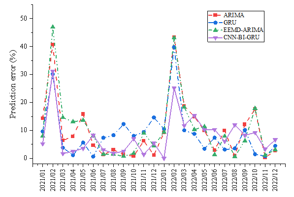
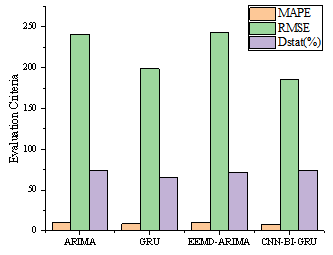
Figure 9 demonstrates the prediction curves of the real value of electricity with the four models ARIMA, GRU, EEMD-ARIMA, and CNN-BI-GRU for renewable electricity. Figure 10 presents the prediction error curves for the four models. Figure 11 displays the three evaluation metrics MAPE, RMSE, Dstat for the four models. Based on these short-period forecast results, we can observer these conclusion as follows.
First, Figure 9 presents a comparison between the actual electricity values and the predictions made by four different models: ARIMA, GRU, EEMD-ARIMA, and CNN-BI-GRU. It is noticeable that while all models follow the trend of the actual values to some extent, they each have varying degrees of accuracy and precision. The short-term nature of the forecast likely introduces significant uncertainty due to the influence of many unpredictable factors that can affect electricity consumption and production on a short scale. Additionally, Figure 10 illustrates the forecasting errors of the same models. It appears that some models have larger spikes in error, potentially indicating moments when the actual values had sudden changes that the models failed to predict accurately. The variability and sudden changes in electricity demand or supply can be difficult for some models to capture, especially in a short-term context. In addition, Figure 11 shows the evaluation metrics MAPE, RMSE, and Dstat. These metrics provide a quantitative measure of the models' performance. The graph suggests that one of the proposed model has a significantly lower MAPE and RMSE, indicating better performance on average compared to the others. Besides, among these four models, the Dstat of the model proposed in this paper is relatively high, which also indicates that the prediction direction of the model proposed in this paper is more accurate.
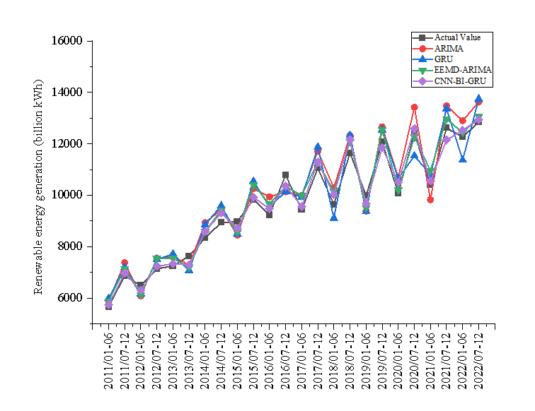
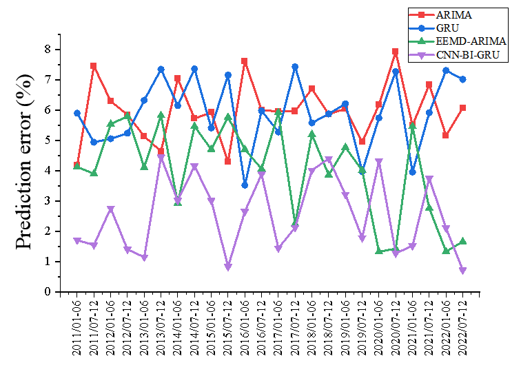
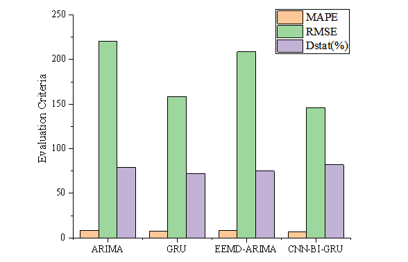
Figure 12 presents the prediction curves of the actual power values by four different models: ARIMA, GRU, EEMD-ARIMA, and CNN-Bi-GRU for renewable electricity. Figure 13 depicts the error curves of these models' predictions. Figure 14 displays the performance of these four models across three evaluation metrics: MAPE, RMSE, and Dstat. Based on the results of these long-term forecasts, we can draw the following conclusions.
Firstly, Figure 12 compares the actual power values with the forecasted values by the four distinct models: ARIMA, GRU, EEMD-ARIMA, and CNN-GRUBI-. These models exhibit trends similar to the actual data in long-term forecasting, demonstrating higher predictive accuracy compared to short-term forecasts. This suggests that the impact of many unpredictable factors is significantly reduced in long-term forecasting. Figure 13 presents the predictive error of these models, indicating that long-term forecasting errors are generally lower than those of short-term forecasts, which underscores the reliability and credibility of long-term predictions. Additionally, the evaluation metrics of MAPE, RMSE, and Dstat shown in Figure 14 provide a quantitative assessment of the models' performance. The proposed model in this study exhibits smaller values in MAPE and RMSE compared to the ARIMA, GRU, and EEMD-ARIMA models, indicating superior average performance. Moreover, the higher Dstat value for the proposed model suggests more accurate predictive directionality.
In addition, we conducted paired sample t-tests to evaluate the performance differences between CNN-Bi-GRU and the baseline models (ARIMA, GRU, EEMD-ARIMA). The t-test results indicate that CNN-Bi-GRU demonstrates statistically significant improvements over ARIMA (p = 0.01), GRU (p = 0.03), and EEMD-ARIMA (p = 0.02), confirming that the observed performance enhancements are not due to random variations but result from the structural optimizations of the proposed model.
For the comparison between CNN-Bi-GRU and ARIMA, the p = 0.01 result suggests a highly significant difference. This indicates that deep learning models can more effectively capture the complex nonlinear characteristics of electricity demand compared to traditional time series methods such as ARIMA. Since ARIMA relies on linear assumptions, it performs well in stable time series forecasting but struggles to generalize when faced with high volatility and multi-factor influences in electricity demand. In contrast, CNN-Bi-GRU overcomes this limitation by utilizing deep feature extraction and bidirectional temporal modeling.
In the comparison between CNN-Bi-GRU and GRU, the p = 0.03 result indicates a statistically significant improvement. This can be attributed to the bidirectional structure of Bi-GRU, which enables the model to consider both past and future information in a time series, whereas unidirectional GRU only leverages historical data for prediction. As a result, GRU has certain limitations in modeling long-term dependencies. Additionally, the integration of CNN enhances feature extraction, allowing CNN-Bi-GRU to outperform GRU in both RMSE and MAPE metrics.
For the comparison between CNN-Bi-GRU and EEMD-ARIMA, the p = 0.02 result confirms a statistically significant performance gain. Although EEMD-ARIMA improves traditional statistical methods by using EEMD to denoise and smooth time series data, it still relies on ARIMA's linear modeling capabilities. This makes it less effective in capturing the complex fluctuations in electricity demand. In contrast, CNN-Bi-GRU leverages CNN to extract local temporal features and utilizes Bi-GRU to model temporal dependencies, providing superior adaptability in handling nonlinear, cyclical, and abrupt changes.
In summary, whether for short-term or long-term demand forecasting of renewable energy, the proposed multimodal information fusion CNN-Bi-GRU model outperforms the ARIMA, GRU, and EEMD-ARIMA models in terms of predictive performance. These experimental results validate the effectiveness of the predictive design scheme proposed in this paper. It is worth noting that the proposed model still has certain limitations when dealing with specific types of data or particular scenarios. For instance, extreme unexpected events, such as power grid failures or abrupt policy changes, may cause significant shifts in historical data patterns. Since the CNN-Bi-GRU model relies on time series features and textual information, it may struggle to quickly adapt to such changes, thereby affecting prediction accuracy. Additionally, data missingness or poor data quality poses a significant challenge. When the input data contains a large number of missing values or anomalies, the model may fail to effectively learn trend features, leading to prediction biases.
This study presents a novel integrated forecasting modeling approach, CNN-Bi-GRU, for short-term and long-term renewable power demand prediction, based on the concept of multimodal information fusion. In this approach, we delve into the analysis of data essential for power demand forecasting and employ the robust feature extraction capabilities of CNNs to extract relevant latent features from both time series and textual data. Subsequently, a concatenation fusion method is applied to organically merge these features, harnessing the complementary nature of information from both modalities. Finally, the fused features are inputted into a Bi-GRU model for prediction. Through comparative experiments with traditional forecasting models and ensemble models, the proposed model exhibits superior directional and level accuracy over widely adopted time series forecasting models, thus effectively validating the superiority of our model in terms of predictive performance. The proposed model is primarily applied to smart grid optimization, electricity market scheduling, and renewable energy generation forecasting. However, challenges remain in practical deployment, including computational costs, data acquisition and quality issues, and extreme unexpected events. Additionally, this study has certain limitations. For instance, the feature extraction module employs a convolutional neural network to extract textual features, making it difficult to interpret the actual significance of the extracted information. Furthermore, the chosen multimodal information fusion method is based on feature-level fusion, which limits the depth of text data mining in this study. Future work will focus on further optimizing the model structure, improving multimodal fusion efficiency, and enhancing the model's anomaly detection capabilities.
 Copyright © 2025 by the Author(s). Published by Institute of Emerging and Computer Engineers. This article is an open access article distributed under the terms and conditions of the Creative Commons Attribution (CC BY) license (https://creativecommons.org/licenses/by/4.0/), which permits use, sharing, adaptation, distribution and reproduction in any medium or format, as long as you give appropriate credit to the original author(s) and the source, provide a link to the Creative Commons licence, and indicate if changes were made.
 IECE Transactions on Emerging Topics in Artificial Intelligence
ISSN: 3066-1676 (Online) | ISSN: 3066-1668 (Print)
Email: [email protected]

Portico
All published articles are preserved here permanently:
https://www.portico.org/publishers/iece/